Download
1 / 25
250 likes | 364 Views
MODELLING REPEATED MEASURES ON FAMILY MEMBERS IN GEOGRAPHICAL AREAS. IAN PLEWIS UNIVERSITY OF MANCHESTER PRESENTATION TO RESEARCH METHODS FESTIVAL OXFORD, 2 JULY 2008. There are research questions in the social sciences that require descriptions and explanations of variability in one or

E N D
MODELLING REPEATED MEASURES ON FAMILY MEMBERS IN GEOGRAPHICAL AREAS IAN PLEWIS UNIVERSITY OF MANCHESTER PRESENTATION TO RESEARCH METHODS FESTIVAL OXFORD, 2 JULY 2008
There are research questions in the social sciences that require descriptions and explanations of variability in one or more outcomes within and between families.
Some of these questions can be addressed by partitioning and modelling: • variation within individuals (when we have repeated measures); • variation between individuals within families (with the appropriate design); • variation between families within areas/neighbourhoods, schools, cross-classifications etc. (with a clustered or spatial design).
The Millennium Cohort Study (MCS), for example, meets these three criteria because, as well as being longitudinal, data are collected from the main respondent (mothers), their partner (if in the household), the cohort child (or children if multiple birth) and older sibs. Also, MCS was originally clustered by ward (although residential mobility reduces the spatial clustering over time).
So we can model ytijk, assumed continuous, where: t = 1…Tijk are measurement occasions (level 1); i = 1…Ijk are individual family members (level 2); j = 1..Jk are families (level 3); k = 1..K are neighbourhoods (level 4). This is the usual nested or hierarchical structure.
For variables that change with age or time, educational attainment for example, we can use a polynomial growth curve formulation:
Do growth rates vary systematically with individual, family and neighbourhood characteristics? We model variation in the random effects bqijk in terms of variables at: • the individual level, e.g. gender, • the family level, e.g. family income, • the neighbourhood level, e.g. Index of Multiple Deprivation.
We might prefer to model the variation in the time-varying outcome in terms of one or more time-varying explanatory variables. For example, we might be interested in how individuals’ smoking behaviour varies as their income changes. This model raises the tricky issue of endogeneity of individual (uijk) and family effects (v0jk) generated by unobserved heterogeneity at these two levels that is correlated with x, especially if we are interested in the causal effect of income on behaviour.
The growth curve and conditional models are compared in, for example: Plewis, Multivariate Behavioral Research, 2001.
These two approaches both ignore the fact that family members have labels: mother, father, oldest sibling etc. Often, we would like to know how the behaviour and characteristics of one family member are related to those of other family members. • The influences of parents on children and children on parents: mental health and behaviour. • The influence of one parent (or, more generally, partner) on another: quitting (or starting) smoking. • The influence of one sibling on others: risky behaviour. • The association of parents’/partners’ characteristics on each other’s behaviour: educational qualifications and health behaviours.
In these cases, a multivariate approach (within a multilevel framework) can be more informative as Raudenbush, Brennan and Barnett, J. Family Psych. (1995) first pointed out.
Their model is based on repeated measures of men and women as members of intact couples: Correlations between males and females within individuals - r(eMeF) - and at the family level - r(u0u1) - can be estimated. The equalities of within and between variances for men and women can be tested. Time varying variables can be introduced if appropriate.
This basic model can be extended to: • Situations where ‘growth’ isn’t obviously applicable, as might be the case for binary and categorical variables (mover-stayer or mixture models). • Couples plus children. • Changing household structures (two parents to one parent for example).
Suppose we have repeated measures of whether (and how much) mothers, fathers and their adolescent children smoke and that we are interested in influences across family members over time, and of educational qualifications (and area of residence) on smoking behaviour.
M, t-1 M, t M, Ed. F, t F, t-1 F, Ed. M, smok A, t A, t-1 F, smok
t = 2..Ti; min(Ti = 3); neighbourhood level omitted for ease of exposition.
The model allows for correlated random effects at the individual level (ui for M, F and A) and also correlated residuals at each occasion (etialso for M, F and A), multivariate Normal in each case.
Estimation and specification issues: • Simultaneity – y2 is predicted by y1 but y2 is a predictor of y3 etc. so we need a FIML estimation method. Not a problem with continuous x and y but perhaps more problematic for non-linear models. MCMC needed? • Autocorrelation structure for level one residuals? E(etet-1) < 0?
Endogeneity of family residuals (ui) – could use y1 as a control for this but then min(Ti) =4. • Missing data – essentially complete case analysis without imputation. • Assumption of Normality for random effects. Clark and Etilé, J. Health Economics, 2006 use a similar model but estimate using a modified EM procedure with non-parametric individual random effects.
Estimates from bivariate probit model: MCS waves 1 and 2,intact couples
Effects of gaining, losing, changing partner – previous research suggests that there are some for smoking but papers have not linked one family member to another. Focus here on women because men generally not followed up in cohort studies. Studies like BHPS might be more informative.
Changes in household structure, MCS, waves 1 to 2 and 1 to 3.
Can accumulate data over time intervals. Can specify more complex models for women who change partners. Expect interactions between δ and other explanatory variables. Single level but can be repeated for women gaining/losing partners more than once.
CONCLUDING REMARKS • Multilevel modeling is a powerful technique for disentangling sources of variation. • Using bivariate (or multivariate) multilevel models for repeated measures data extends the range of hypotheses about within household influences on behaviour that can be tested. • It is important to model what actually happens to households over time and not always to rely on analyses of intact couples. • What hypotheses might we consider for neighbourhood effects?
POSSIBLE EXTENSIONS • The problem of limited dependent variables, especially for measures of amount smoked which is censored at zero. Multilevel extensions of Tobit, mixture or Heckman selection models might be useful here. • Combining growth curve models with models for non-smokers. For example, Carlin et al. (Biostatistics, 2001) suggest a mixture model.