Equality Constraints (Jacobian Method)
Equality Constraints (Jacobian Method). Constrained Derivatives (Jacobian) Method. Consider The following Problem: Minimize z = f(X) Subject to g(X) = 0 Where X = (x l , x 2 ,… , x n ) g = (g 1 , g 2 ,… , g m ) T

Equality Constraints (Jacobian Method)
E N D
Presentation Transcript
Constrained Derivatives (Jacobian) Method Consider The following Problem: Minimize z = f(X) Subject to g(X) = 0 Where X = (xl, x2,… , xn ) g = (g1, g2,… , gm)T • The functions f(X) and g(X), i = 1,2, ... , m, are twice continuously differentiable. • The idea of using constrained derivatives is to develop a closed-form expression for the first partial derivatives of f(X) at all points that satisfy the constraints g(X) = 0. • The corresponding stationary points are identified as the points at which these partial derivatives vanish.
Consider f(xl, x2) This function is to be minimized subject to the constraint g1(xl, x2) = x2 -b= 0 (x2=b) • b is a constant. • A, B, and C represents the values of f(xl,x2) for which the given constraint is always satisfied. • The constrained derivatives method defines the gradient of f(xl,x2) at any point on the curve ABC. • Point B at which the constrained derivative vanishes is a stationary point for the constrained problem.
By Taylor's theorem, for (X + Δ X) in the feasible neighborhood of X, we have: f(X + Δ X) - f(X) = ∇ f(X) Δ X + O(Δ xj2) g(X + Δ X) - g(X) = ∇ g(X) Δ X + O(Δ xj2) Δxj→0 ∂f(X) = ∇f(X) ∂x and ∂g(X) = ∇g(X) ∂x
For feasibility, we must have g(X) = 0 ∂g(X) = 0 and it follows that ∂ f(X) - ∇f(X) ∂ x = 0 ∇g(X) ∂ x = 0 This gives (m+1) equations in (n+1) unknowns, ∂f(X) and ∂X. Note that ∂f(X) is a dependent variable, and hence is determined as soon as ∂X is known. This means that, in effect, we have m equations in n unknowns.
If m > n, at least (m - n) equations are redundant. Eliminating redundancy, the system reduces to m ≤ n. If m = n, the solution is ∂x= 0, and X has no feasible neighborhood, which means that the solution space consists of one point only. Define x = (Y, Z) such that y = (Y1 ,Y2,···,Ym), Z = (Z1, Z2,···,Z n-m)
The vectors Y and Z are called the dependent and independent variables, respectively. Rewriting the gradient vectors of f and g in terms of Y and Z, we get • ∇f(Y, Z) = (∇y f, ∇z f) • ∇g(Y, Z) = (∇y g, ∇z g) Define J= ∇y g = C= ∇z g =
Jmx m is called the Jacobian matrix and Jm x n-m the control matrix. The Jacobian J is assumed nonsingular. This is always possible because the given m equations are independent by definition. The components of the vector Y must thus be selected from among those of X such that J is nonsingular.
The original set of equations in ∂ f(X) and ∂ x may be written as ∂ f(Y, Z) = ∇yf ∂y + ∇zf ∂z And J ∂Y = -C∂Z Because J is nonsingular, its inverse J-1 exists. Hence, Substituting for ∂ Y in the equation for ∂ f(X) gives ∂f as a function of ∂ Z-that is: ∂f(Y, Z) = (∇zf - ∇yfJ-1 C) ∂Z From this equation, the constrained derivative with respect to the independent vector Z is given by ∇c f = = ∇z f - ∇y f J-1 C where ∇cf is the constrained gradient vector of f with respect to Z. Thus, ∇cf(Y, Z) must be null at the stationary points.
The Hessian matrix will correspond to the independent vector Z, and the elements of the Hessian matrix must be the constrained second derivatives. To show how this is obtained, Let ∇c f = ∇Z f – WC It thus follows that the ith row of the (constrained) Hessian matrix is . Notice that W is a function of Y and Y is a function of Z. Thus, the partial derivative of ∇cf with respect to Zi is based on the following chain rule: =