Conjugate Gradient and Linear Equality Constraints
220 likes | 369 Views
Conjugate Gradient and Linear Equality Constraints . Lecture III. A Slightly More Complicated Problem. Starting with a hyperbolic tangent production function We define the profit function as. As a starting point, we assume Starting with some feasible step s 1. If we let.

Conjugate Gradient and Linear Equality Constraints
E N D
Presentation Transcript
Conjugate Gradient and Linear Equality Constraints Lecture III
A Slightly More Complicated Problem • Starting with a hyperbolic tangent production function • We define the profit function as
As a starting point, we assume • Starting with some feasible step s1
Given that B1 is the identity matrix • Thus, in this case we have
Next, to update the Hessian matrix following the BFGS algorithm we have
Updating the solution, next we have the gradient at the new solution as
R-Code fr <- function(b){-15/2*(1+tanh(-0.50+0.2625*b[1]+0.3125*b[2]+0.3500*b[3]- 0.0025*b[1]*b[1]-0.0028*b[2]*b[2]-0.0025*b[3]*b[3]+ 0.00035*b[1]*b[2]+0.00028*b[1]*b[3]+0.000032*b[2]*b[3])) +0.375*b[1]+0.450*b[2]+0.475*b[3]} dfr <- function(b){ dd <- cosh(0.50-0.2625*b[1]-0.3125*b[2]-0.3500*b[3]+0.0025*b[1]*b[1]+0.0028*b[2]*b[2]+ 0.0025*b[3]*b[3]-0.00035*b[1]*b[2]-0.00028*b[1]*b[3]-0.000032*b[2]*b[3]) as.matrix(cbind(0.375+(15/2)*(-0.2625+0.00500*b[1]-0.00035*b[2]-0.00028*b[3])/(dd*dd), 0.450+(15/2)*(-0.3125-0.00035*b[1]+0.00560*b[2]-0.000032*b[3])/(dd*dd), 0.475+(15/2)*(-0.3500-0.00028*b[1]-0.000032*b[2]+0.0050*b[3])/(dd*dd)))} b0 <- cbind(1.0,1.0,1.0) res.fr <- optim(b0,fr,dfr,method="BFGS") print(res.fr)
Results $par [,1] [,2] [,3] [1,] 1.062955 0.4756912 4.537824 $value [1] -11.46800 $counts function gradient 28 23 $convergence [1] 0 $message NULL
Starting with a simple 2*3 example, assume that we have the matrix equation • Note that by row operations the A matrix can be transformed to
This expression implies the following homogeneous relationships: • Setting x3=1 yields
Or in vector form: • Next we confirm that z is the nullspace.
We do this by confirming that both vectors of the matrix are orthogonal to the nullspace:
Implications of the nullspace: • Start by defining a feasible solution:
Next, we would like to generate another feasible point based on this solution and the nullspace matrix: • Letting yields p = 5