Download

1 / 21
230 likes | 406 Views
Genetic Regulatory Network Inference. Russell Schwartz Department of Biological Sciences Carnegie Mellon University. Why Study Network Inference?. It can help us understand how to interpret and when to trust biological networks

E N D
Genetic Regulatory Network Inference Russell Schwartz Department of Biological Sciences Carnegie Mellon University
Why Study Network Inference? It can help us understand how to interpret and when to trust biological networks It is a model for many kinds of complex inference problems in systems biology and beyond It is a great example of a machine learning problem, a kind of computer science central to much work in biology Network inference is a good way of thinking about issues in data abstraction central to all computational thinking
Our Assumptions + + + - + Cro cI - + * genes conditions We will focus specifically on transcriptional regulatory networks, assuming no cycles We will assume, at least initially, that our data source is a set of microarray gene expression values *Clustered gene expression data from NCBI Gene Expression Omnibus (GEO), entry GSE1037: M. H. Jones et al. (2004) Lancet 363(9411):775-81.
Intuition Behind Network Inference 1 1 1 1 1 genes 2 2 2 2 2 3 3 3 3 3 4 4 4 4 4 conditions 1 1 + - 1 + - 2 3 2 3 - - … 2 3 - 1 1 + + - - 4 2 3 2 3 - correlated expression implies common regulation that intuition still leaves a lot of ambiguity
Why Is Intuition Not Enough? … • Models are ambiguous: • Data are noisy: • Data are sparse: * 1 1 1 3 3 2 3 2 2 4 4 4 *Clustered gene expression data from NCBI Gene Expression Omnibus (GEO), entry GSE1037: M. H. Jones et al. (2004) Lancet 363(9411):775-81.
A Next Step Beyond Intuition: Assuming a Binary Input Matrix conditions gene 1 1 1 0 0 1 1 1 0 gene 2 1 1 1 1 0 0 1 0 gene 3 1 0 0 0 0 1 0 0 gene 4 0 0 0 0 0 1 0 1 1 4 We will assume for the moment that genes only have two possible states: 0 (off) or 1 (on) We will also assume that we want to find directionality but not strength of regulatory interactions: 2 3
Making it Even Simpler: Two Genes conditions gene 1 1 1 0 0 1 1 1 0 gene 2 1 1 1 0 0 1 0 1 2 1 2 1 1 2 model 2 “G2 regulates G1” model 3 “G1 and G2 are independent” model 1 “G1 regulates G2” Only three possible models to consider
Judging a Model: Likelihood Complicated inference problems like this are commonly described in terms of probabilities We want to infer a model (which we will call M) using a data set (which we will call D) Problems like this are commonly posed in terms of maximizing a likelihood function: We read this as “probability of the data given the model,” i.e., the probability that a given model would generate a given data set
What is the Probability of a Microarray? Pr{ }= Pr{ }x Pr{ }x Pr{ }x Pr{ }x Pr{ }x Pr{ }x Pr{ }x Pr{ } 1 1 0 0 1 1 1 0 1 1 1 0 0 1 1 0 We can describe the probability of a microarray as the product of the probabilities of all of its individual measurements:
What is the Probability of One Measurement on a Microarray? 1 0 1 0 Pr{ } =Pr{ }x Pr{ }x Pr{ }x Pr{ }x Pr{ }x Pr{ }x Pr{ }x Pr{ } =5/8 x 5/8 x 3/8 x 3/8 x 5/8 x 5/8 x 5/8 x 3/8 = 0.00503 1 1 0 0 1 1 1 0 1 1 1 0 0 1 1 0 • We can estimate Pr{ } and Pr{ } by counting how often each individual value occurs: • Pr{ } = 5/8 • Pr{ } = 3/8 • Therefore:
Evaluating One Model gene 1 1 1 0 0 1 1 1 0 data D = gene 2 1 1 1 0 0 1 0 1 model M = 1 2 Pr{D|M} = Pr{ } x Pr{ } = 0.00503 x 0.00503 = 2.5 x 10⁻⁵ 1 1 0 0 1 1 1 0 1 1 1 0 0 1 0 1
Adding in Regulation gene 1 1 1 0 0 1 1 1 0 2 1 gene 2 1 1 1 1 0 0 1 0 Pr{G2= |G1= } = 1/5 Pr{G2= |G1= } = 2/3 0 1 0 0 Pr{G2= |G1= } = 4/5 Pr{G2= |G1= } = 1/3 0 1 1 1 How do we evaluate output probabilities for a regulated gene? We need the notion of conditional probability: evaluating the probability of gene 2’s output given that we know gene one’s output:
Evaluating Another Model gene 1 1 1 0 0 1 1 1 0 data D = gene 2 1 1 1 0 0 1 0 1 model M = 1 2 Pr{D|M} = Pr{ } x Pr{ | } = 0.00503 x (1/5 x 4/5 x 2/3 x 1/3 x 4/5 x 4/5 x 4/5 x 2/3) = 6.1 x 10⁻⁵ 1 1 0 0 1 1 1 0 1 1 1 0 0 1 0 1 1 0 0 1 1 1 0 1
Evaluating Another Model gene 1 1 1 0 0 1 1 1 0 data D = gene 2 1 1 1 0 0 1 0 1 model M = 1 2 Pr{D|M} = Pr{ | } x Pr{ } = (1/5 x 4/5 x 2/3 x 1/3 x 4/5 x 4/5 x 4/5 x 2/3) x 0.00503 = 6.1 x 10⁻⁵ 1 1 1 1 1 0 0 1 1 1 0 0 0 1 0 1 1 1 1 0 0 1 0 1
Comparing the Models for Two Genes 1 1 0 0 1 1 1 0 Pr{ | } = 2.5 x 10⁻⁵ 1 2 1 1 1 0 0 1 0 1 1 1 0 0 1 1 1 0 Pr{ | } = 6.1 x 10⁻⁵ 1 2 1 1 1 0 0 1 0 1 1 1 0 0 1 1 1 0 Pr{ | } = 6.1 x 10⁻⁵ 1 2 1 1 1 0 0 1 0 1 Conclusion: Knowing the expression of gene 1 helps us predict the expression of gene 2 and vice versa; we can suggest there should be an edge between them but cannot decide the direction it should take
Generalizing to Many Genes 1 1 0 0 1 1 1 0 1 4 1 1 1 0 0 1 0 1 Pr{ | } = Pr{ } x Pr{ | } x Pr{ | , } x Pr{ | } 1 0 0 0 0 1 0 0 2 3 0 0 0 0 1 0 1 0 1 1 0 0 1 1 1 0 1 1 1 0 0 1 0 1 1 0 0 1 1 1 0 1 1 0 0 0 0 1 1 1 0 0 1 1 1 0 0 0 1 1 1 0 0 1 0 1 1 0 0 0 0 1 0 0 0 0 0 0 1 0 1 0 The same basic concepts let us evaluate the plausibility of any regulatory model This is known as a Bayesian graphical model
Adding Prior Knowledge 1 1 0 0 1 1 1 0 1 1 4 1 1 1 0 0 1 0 1 Pr{ | } x Pr{ } x Pr{ } x Pr { } x Pr { } x … 1 0 0 0 0 1 0 0 2 3 2 0 0 0 0 1 0 1 0 1 1 2 4 3 3 We can also build in any prior knowledge we have about the proper model (e.g., from the literature) We can use that knowledge by simply multiplying each likelihood by our prior confidence in its validity:
Adding in Other Data Types 1 1 1 0 0 1 1 1 0 Pr{ , ACGATCTCA… | } = Pr{ | } x Pr{ACGATCTCA … | } 1 1 1 0 0 1 0 1 2 1 1 1 0 0 1 1 1 0 1 1 1 0 0 1 0 1 2 1 Evaluate as before 2 We can also incorporate other pieces of evidence in much the same way Example: suppose we have microarrays and TF binding site predictions: Evaluate by a binding site prediction method (e.g., PSSM)
Moving from Discrete to Real-Valued Data 1.5 0.4 -0.3 -1.2 -1 0 1 1.5 0.4 -0.3 -1.2 Pr{ } = We can also drop the need for discrete (on or off) data by making an assumption of how values vary in the absence of regulation, e.g., Gaussian:
Finding the Best Model • We now know how to compare different network models, but finding the best model is not easy; far too many possibilities to compare them all • Algorithms for model inference is a more complex topic than we can cover here, but there are some general approaches to be aware of • optimization: many specialized methods exist for finding the best model without trying everything; solving hard problems of this type is a core concern in computer science • sampling: there are also many specialized methods for randomly generating solutions likely to be “good” and seeing what model features are preserved across most solutions; this is a core concern of statisticians
Network Inference in Practice The methods covered here are the key ideas behind how people really infer networks from complex data The practice is usually more complicated, though: many kinds of data sources, specialized prior probabilities, lots of algorithmic tricks needed to get good results If you really want to know the details, these topics are typically covered in a class on machine learning