Download
1 / 42
420 likes | 546 Views
This presentation delves into the simulation of granular materials, particularly their unique physical properties and behaviors. It examines the challenges of simulating granular interactions, including energy loss during collisions and complex particle dynamics. A proposed model outlines how granular materials can be represented as discrete particles or fluid-like substances, with various applications in engineering design and entertainment industries. Key topics include stress behaviors, yield conditions, and efficient collision detection methods, alongside practical examples such as avalanches and sand simulation in films.

E N D
Sand Simulation Abhinav Golas COMP 768 - Physically Based Simulation Final Project Presentation
Motivation • Movies, games • Engineering design – grain silos • Avalanches, Landslides Spiderman 3 The Mummy www.stheoutlawtorn.com
Overview • What are Granular Materials? • Proposed Model • Actual Progress
Overview • What are Granular Materials? • Proposed Model • Actual Progress
What are Granular Materials? • A granular material is a conglomeration of discrete solid, macroscopic particles characterized by a loss of energy whenever the particles interact (Wikipedia) • Size variation from 1μm to icebergs • Food grains, sand, coal etc. • Powders – can be suspended in gas
What are Granular materials? • Can exist similar to various forms of matter • Gas/Liquid – powders can be carried by velocity fields • Sandstorms • Liquid/Solid – similar to liquids embedded with multiple solid objects • Avalanches, landslides • Hourglass • Similar to viscous liquids
Why the separate classification? • Behavior not consistent with any one state of matter • Can sustain small shear stresses – stable piles • Hydrostatic pressure achieves a maximum • Particle interactions lose energy • Collisions approach inelastic • Infinite collisions in finite time – inelastic collapse • Inhomogeneous and anisotropic • Particle shape and size inhomogeneous Granular solids, liquids, and gases – Jaeger et al.
Understanding the behavior - Stress y y z z • Stress • At equilibrium – matrix is symmetric – 6 degrees of freedom • Pressure for fluids – tr(σ)/ 3 Shear Normal
Stress • Different matrix for different basis – need invariants • Pressure! – I0 • Deviatoric invariants – Invariants based on J1,J2 • Eigen values? – called principle stresses
Understanding the behavior • Why can sand sustain shear stress? • Friction between particles • When does it yield? – yield surface/condition
Yield surface • Many surfaces – suitable for different materials • Mohr Coulomb surface with Von-Mises equivalent stress – f(I0, J1) • Condition for stability/rigidity: • sinΦ – coefficient of friction
So why is it difficult to simulate? • Scale - >10M particles • Nonlinear behavior – yield surface • Representation – discrete or continuum?
Simulation • Depends on what scenario to simulate • Discrete particles – Particle-Based Simulation of Granular Materials, Bell et al. • Continuum – Animating Sand as a Fluid, Zhu et al.
Particle-Based Simulation of Granular Materials • Use a particle system with collision handling • Define objects in terms of spheres • Need to define per sphere pair interaction forces • Collision system based on Molecular Dynamics • Allow minor spatial overlap between objects
Sphere pair interaction • Define overlap(ξ), relative velocity(V), contact normal(N), normal and tangential velocities(Vn, Vt), rate of change of overlap(V.N) • Normal forces • kd : dissipation during collisions, kr : particle stiffness • Best choice of coefficients: α=1/2, β=3/2 • Given coefficient of restitution ε, and time of contact tc, we can determine kd and kr
Sphere pair interaction • Tangential forces • These forces cannot stop motion – require true static friction • Springs between particles with persistent contact? • Non-spherical objects
Solid bodies • Map mesh to structure built from spheres • Generate distance field from mesh • Choose offset from mesh to place spheres • Build iso-surface mesh (Marching Tetrahedra) • Sample spheres randomly on triangles • Let them float to desired iso-surface by repulsion forces • D=sphere density, A=triangle area, R=particle radius, place particles, 1 more with fractional probability
Solid bodies • K – interaction kernel, P – Position of particle, V – velocity of particle, Φ – distance field • Rigid body evolution • Overall force = Σ forces • Overall torque = Σ torques around center of mass
Efficient collision detection • Spatial hashing • Grid size = 2 x Maximum particle radius • Need to look at 27 cells for each particle O(n) • Not good enough, insert each particle into not 1, but 27 cells check only one cell for possible collisions • Why better? • Spatial coherence • Particles moving to next grid cell, rare (inelastic collapse) • Wonderful for stagnant regions
Advantages/Disadvantages • The Good • Faithful to actual physical behavior • The Bad and the Ugly • Computationally intensive • Small scale scenes • Scenes with some “control” particles
Animating Sand as a Fluid • Motivation • Sand ~ viscous fluids in some cases • Continuum simulation • Bootstrap additions to existing fluid simulator • Why? • Simulation independent of number of particles • Better numerical stability than rigid body simulators
Fluid simulation? what’s that? v • Discretize 3D region into cuboidal grid • 3 step process to solve Navier Stokes equations • Advect • Add body forces • Incompressibility projection • Stable and accurate under CFL condition u p, ρ u v
Extending our fluid simulator • Extra things we need for sand • Friction (internal, boundary) • Rigid portions in sand • Recall • Stress • Yield condition
Calculating stress • Exact calculation infeasible • Smart approximations • Define strain rate – D = d/dt(strain) • Approximate stresses • Rigid • Fluid
The algorithm in a nutshell • Calculate strain rate • Find rigid stress for cell • Cell satisfies yield condition? • Yes – mark rigid, store rigid stress • No – mark fluid, store fluid stress • For each rigid connected component • Accumulate forces and torques • For fluid cells, subtract friction force
Yield condition • Recap • Can add a cohesive force for sticky materials
Rigid components • All velocities must lie in allowed space of rigid motion (D=0) • Find connected components – graph search • Accumulate momentum and angular momentum • Ri – solid region, u – velocity, ρ – density, I – moment of inertia Rigid Fluid: Animating the Interplay Between Rigid Bodies and Fluid, Carlson et al.
Friction in fluid cells • Update cell velocity • Boundary conditions • Normal velocity: • Tangential velocity:
Representation • Defining regions of sand • Level sets • Particles • Allow improved advection • Hybrid simulation • PIC – Particle In Cell • FLIP – FLuid Implicit Particle
Advantages/Disadvantages • Advantages • Fast & stable • Independent of number of particles – large scale scenes possible • Disadvantages • Not completely true to actual behavior • Detail issues – smoothing in simulation, surface reconstruction
Overview • What are Granular Materials? • Proposed Model • Actual Progress
Proposed Model • Minimization problem • Inelasticity -> stress tries to minimize kinetic energy • Constraints • Friction, yield condition • Boundary conditions • Unilateral incompressibility
Proposed Model • Friction • Nice, but not linear – Frobenius Norm • Infinity/1 Norm – linear • Unilateral Incompressibility • Boundary conditions
Problems • Friction not orthogonal • LCP bye bye • KKT solver slow • Iterative solvers • LCP for unilateral incompressibility, boundary conditions • Friction checking after that • Recurse till convergence
Overview • What are Granular Materials? • Proposed Model • Actual Progress
Actual progress • Boundary cases! • 90% of all effort in writing fluid solver • Minor details • Particle reseeding / preventing clumping • Continuity of stress field • Parameter tuning
Actual progress • Running implementation of “Animating Sand as a Fluid”, Zhu et al. • 3D real-time – albeit with simple rendering • Takes care of friction • Rigid, fluid cases • Boundary cases – tangential contact friction • Variational formulation – “Variational Fluids”, Bridson and Batty
Implementation • Grids coupled with particles • Particles dictate fluid density • One way velocity mapping – need ghost fluids for proper 2 way mapping • Grid based advection • Variational model – better interaction handling with non-axis-aligned objects • Rigid projection
Actual progress • The nitty-gritty • Implemented 3D fluid solver from scratch • Particle System reused from previous assignments • Rigid projection – “Rigid Fluids” • Variational pressure solve – equality constraints
Pluses/Minuses? • Issues • Bugs – known and unknown remain • LCP solver couldn’t be completed in time – no unilateral incompressibility, improved contact • Iterative testing couldn’t be done • Pluses • 3D fluid simulator working • With minor fixes – should be perfectly functional
References • Granular Solids, Liquids, and Gases – Jaeger et al.Review of Modern Physics ’96 • Particle-Based Simulations of Granular Materials – Bell et al., Eurographics ‘05 • Animating Sand as a Fluid – Zhu et al.SIGGRAPH ‘05 • Rigid Fluid: Animating the Interplay Between Rigid Bodies and Fluid – Carlson et al.SIGGRAPH ’04
References • A Fast Variational Framework for Accurate Solid-Fluid Coupling – Batty et al.SIGGRAPH 2007