Download
1 / 37
370 likes | 389 Views
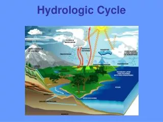
This article examines the hydrologic cycle and water balance in Florida, including rainfall, surface runoff, evapotranspiration, and groundwater storage. It explores the impact of forest management on water yield and nutrient export. Stream patterns and watershed networks are also discussed.

E N D
Florida Water Facts • Surface Area = 170,452 km2 • Average Rainfall = 140 cm (55”) • Total Annual Rain = 238 billion m3(62.6 trillion gallons) • River and Stream = 51,858 miles • Largest River = Apalachicola (Q = 25,000 ft3/s = 22 km3/yr) • Lake Area = 12,100 km2 • Springs ~ 8 billion gallons/ day • Groundwater supplies 95% of water • 7.2 billion gallons/day; 80% to S. Florida • Low relief – travel time for water (rainfall to sea) can be decades
The Hydrologic Check-Book • Mass Balance • Water mass is conserved • Therefore: Water In = Water Out • Sources • Rain, Snow, Groundwater, Human Effluent • Sinks • Ground, River, Atmosphere, Humans • Stores • Wetlands, Lakes, Rivers, Soil, Aquifers
The Water Budget (Exam 1) INFLOW OUTFLOW P= Q + ET + G + ΔS Precipitation Surface runoff Evapotranspiration Groundwater Storage
Annual Water Budget - Flatwoods Transpiration (~ 70 cm) Interception (~ 30 cm) Rainfall (~ 140 cm) Surface Runoff (~ 3 cm) Infiltration to Deep Aquifer (~5 cm, though upto ~ 40 cm) Subsurface Runoff (~ 32 cm)
Annual Water Budget – Ag Land Transpiration (~ 80 cm) Interception (~ 15 cm) Rainfall (~ 140 cm) Surface Runoff (~ 20 cm) Subsurface Runoff (~ 20 cm) Infiltration to Deep Aquifer (~5 cm, in areas much higher)
Annual Water Budget – Urban Land Rainfall (~ 140 cm) Interception (~ 20 cm) Transpiration (~ 50 cm) Surface Runoff (~ 60 cm) Subsurface Runoff (~ 5 cm) Infiltration to Deep Aquifer (~ 2 cm)
Changes in Internal Stores • ΔStorage = Inputs – Outputs • Usually easy to measure (e.g., lake volume) In > Out ? Out > in ? In = Out ? What if Inmeasured > Outmeasured AND water level is falling?
Rules of Water Balances • Water balance terms must be in common units • (usually meters depth over the watershed area). • Precipitation and ET measured in depth (m/yr) • Water flows measured as volumes (m3/yr). Volume = Depth x Area Depth = Volume / Area
An Even Simpler Water Budget • Budyko Curve shows annual catchment hydrology • Can neglect G and ΔS, focus on ET (P ~ ET + Q) • Aridity index on the x-axis (potential ET:rain) • Evaporative index on the y axis (actual ET:rain)
Catchment Water Balance • Area = 100 ha (10,000 m2 per ha) • Annual Measurements: • Rainfall = 2 m (tipping-bucket rain gage) • Surface outflow (Q) = 20,000,000 m3 (weir) • ET = 1.5 m (evaporation pan) • Groundwater = 10,000,000 m3 (shallow wells) • Assume ΔS=0
Budget: P= Q + ET + G + ΔS • Area = 100 ha; 1 ha = 10,000 m2 • P = 2.0 m • Q = 20,000,000 m3/(100 ha * 10,000 m2/ha) = 0.2 m • ET = 1.5 m • G = 10,000,000 m3/(100 ha * 10,000 m2/ha) = 0.1 m • ∆S = 0 • 2.0 = 0.2 + 1.5 + 0.1 + 0 (?!)
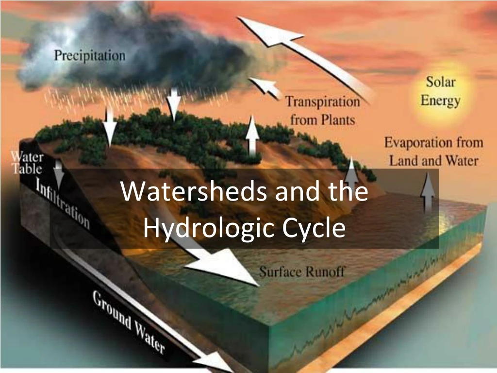
Watersheds • A land area from which all rainfall drains to the same point. • The “watershed” is technically the divide between two such areas (called basins)
Delineating Watersheds • Identify outlet point • Identify high points • Link high pts crossing contour lines at right-angles 2 3 1
Why Watersheds? • Control boundaries • Water that falls either comes out the bottom or is abstracted • Imagine a water budget if you weren’t sure where the water was going… P + Qin1 + Qin2 = Qout1 + Qout2 + ET + G1 + G1 + ΔS
Experimentation – Paired Watersheds • What is the effect of forest management on: • Water yield • Sediment yield • Nutrient export • Water temperature • Time of transport
Paired Watershed Study of Forest Harvest Effects on Peakflows LOGGING ROAD BUILDING Beschta et al. 2000 – H.J. Andrews Experimental Forest (OR)
Does watershed delineation work in Florida? • Low-relief • Delineation of boundaries hard • In parts of Florida, water flows depend on: • where it rained, • where the wind is blowing and • where people put the canals and roads • National contour maps too coarse (5 ft) • Roads act as flow delineators ????
Paired Watersheds in Florida • Shown that (Riekerk 1983): • High intensity logging increased water yields by 250% • Low intensity logging increased water yields 150% • Clear cutting altered nutrient export rates • All forest operations (fire?) were less than urbanization (much more on this later)
Stream Patterns • Dendritic patterns follow Strahler Order • 1st order is unbranched • 2nd order occurs when two 1st order reaches converge • Increased order requires convergence of two reaches of the same order • What are springs?
Network Forms • Regional landform dictates shape • Regional geology dictates drainage density • Regional climate (rainfall) dictates density and maturation rate
Watershed Networks • Mass transport is optimal at minimum work • Reach and network scales at the SAME time • Necessary conditions for dendritic drainage • Minimal energy expenditure at any link in the network • Equal Energy Expenditure per unit area • Minimum Energy Expenditure in the Network as a whole Rodriguez-Iturbeet al. (1992) - WRR
Water Convergence Across Scales - St Johns River Basin - Ocklawaha River Basin - Orange Creek Sub-Basin - Newnans Lake Watershed - Hatchett Creek Watershed - ACMF “Hillslope” - Lake Mize catchment
Lake Mize hillslope Conference Center Lake Mize
Austin Cary Forest Waldo Road Lake Mize Hatchett Creek
Hatchet Creek Catchment Hatchett Creek
Newnans Lake Watershed Santa Fe Swamp Hatchett Creek Gainesville Lake Forest Creek Newnans Lake Prairie Creek
Orange Creek Basin Newnans Lake Paynes Prairie Lochloosa Lake Orange Lake
Ocklawaha RiverBasin Orange Creek Basin Rodman Reservoir Silver Springs Ocklawaha River Lake Apopka
St. Johns River Basin (and Water Management District) St. Johns River
Next Time… • Precipitation • Where it falls • When it falls • How it’s made • How we measure it