Download
1 / 49
520 likes | 570 Views
Explore modeling findings from the Lake Ontario Contaminant Monitoring Workshop in 2007, focusing on mercury deposition impact, source attribution, and multi-media framework development for ecological assessment. Discover the interplay of atmospheric and aquatic mercury cycling in the Great Lake region.

E N D
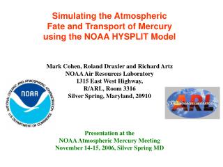
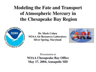
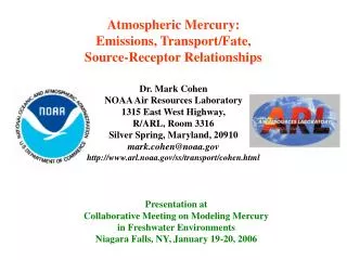
Atmospheric Fate and Transport of Mercury Mark Cohen NOAA Air Resources Laboratory 1315 East West Highway, R/ARL, Room 3316 Silver Spring, Maryland, 20910, USA mark.cohen@noaa.gov http://www.arl.noaa.gov/ss/transport/cohen.html Lake Ontario Contaminant Monitoring & Research Workshop Planning for the 2008 Cooperative Monitoring Year - Contaminants Component – Grand Island Holiday Inn, Grand Island, New York March 27 & 28, 2007
Thanks, John! Standing (from left): Eric Uram, Gary Foley, John McDonald, Greg Mierle, Sheng-Wei Wang; Kneeling (from left): Chris Knightes, Elsie Sunderland, Wolfgang Scheider, Mark Cohen At the Lake Ontario Contaminant Monitoring, Modeling & Research Workshop, Grand Island, NY, March 27-28, 2007
MANY THANKS TO: • Gary Foley, J. David Mobley, Elsie Sunderland, Chris Knightes (EPA); Panos Georgopolous and Sheng-Wei Wang (EOSHI Rutgers Univ); John McDonald (IJC): funding and collaboration on multimedia Hg modeling • David Schmeltz, Gary Lear, John Schakenbach, Scott Hedges, Rey Forte (EPA): funding and collaboration on Hg models and /measurements, including new EPA-NOAA Hg monitoring site at Beltsville, MD. • David Ruple, Mark Woodrey (Grand Bay NERR), Susan White , Gary Matlock, Russell Callender, Jawed Hameedi (NOAA), and Durwin Carter (U.S. Fish and Wildlife Service): collaboration at NOAA Grand Bay NERR atmospheric monitoring site • Anne Pope and colleagues (EPA): U.S. mercury emissions inventory • David Niemi, Dominique Ratte, Marc Deslauriers (Environment Canada): Canadian mercury emissions inventory data • Mark Castro (Univ. Md, Frostburg), Fabien Laurier (Univ Md Ches Biol Lab), Rob Mason (Univ CT), Laurier Poissant (Envr Can): ambient Hg data for model evaluation • Roland Draxler, Glenn Rolph, Rick Artz (NOAA):HYSPLIT model and met data • Steve Brooks, Winston Luke, Paul Kelley (NOAA) : ambient Hg data
atmospheric chemistry inter-converts mercury forms Hg(0) Hg from other sources: local, regional & more distant Hg(II) Hg(p) emissions of Hg(0), Hg(II), Hg(p) Surface exchange with the watershed Surface exchange with the lake 4
Objectives and Rationale of Atmospheric Modeling in Conjunction with Great Lake Multi-Compartment Mercury Modeling Project • Estimate deposition amount of different mercury species and/or forms to different regions of Lake Ontario lake surface and watershed, for use in ecological assessment and modeling • dry deposition generally estimated with models • modeling can help fill in spatial gaps between measurement sites • modeling can help estimate deposition for other times • past • future (for different emissions scenarios) • Estimate source attribution for deposition of different mercury species and/or forms to different regions of Lake Ontario lake surface and watershed, including estimation of the relative importance of: • different source regions (local, regional, national, continental, global) • different jurisdictions (different states and provinces) • anthropogenic vs. natural emissions • different anthropogenic source types (power plants, waste incin., etc) 5
Largest mercury sources in U.S. and Canadian air emissions inventories (~1999-2000) Source of emissions data: U.S. EPA and Environment Canada
Some preliminary results for the atmospheric deposition impact of U.S. and Canadian anthropogenic mercury air emissions sources on Lake Ontario
Largest modeled atmospheric deposition contributors to Lake Ontario based on 1999-2000 emissions
Modeled atmospheric mercury deposition to Lake Ontario from U.S. and Canadian source sectors based on 1999-2000 emissions
Top 25 Contributors to 1999 Hg Deposition Directly to Lake Ontario
Many uncertainties in these earlier results… How to refine modeling and link with other models in a multi-media framework?
Hg(0) Hg(II) Hg(p) For Lake Ontario: How to link the atmospheric model and the aquatic fate/cycling model? 12
Surface exchange of Hg(0) from Lake Ontario may not have large impact on overall atmospheric Hg fate-transport (?) Hg(0) Hg(II) Hg(p) Upward Flux of Hg(2) and Hg(p) is probably small Hg(0) Hg(2) Hg(p) The precise specification of surface exchange of Hg(0) may not have large impact on methyl-mercury production (???) It may turn out that dynamic, run-time linkage between lake and atmosphere is not critical for Hg (?) (we will see…) Air-Water Interface – at the boundary between the atmospheric model (over the lake) and the lake fate and cycling model 13
Inputs to Model For model evaluation, emissions and meteorology must be for the same time period as ambient measurement data meteorology emissions Atmospheric Mercury Model atmospheric chemistry wet deposition phase partitioning surface exchange Model Evaluation Speciated ambient concentration data Wet deposition data Model Outputs Wet and dry deposition of different mercury species to lake and watershed Source attribution information for deposition emissions Speciated ambient concentration data 14
2000 Global Inventory New York inventory 1995 Canada Inventory 2000 Canada Inventory Ontario inventory ? 1999 US Inventory 2002 US Inventory ? speciated atmospheric Hg measurements at site x Hypothetical – just for illustration purposes speciated atmospheric Hg measurements at site y speciated atmospheric Hg measurements at site z For model evaluation, inventory must be accurate and for same period as measurements (a big challenge!) 95 96 97 98 99 00 01 02 03 04 05 06 07 08 09 10 11 12 13 14 15 15
RGM emissions (~1999) in the Lake Ontario region “RGM” = Reactive Gaseous Mercury, the form of atmospheric mercury most readily deposited Lake Ontario 16 Source of emissions data: U.S. EPA and Environment Canada
RGM emissions (~1999) in the Lake Ontario region, and Mercury Deposition Network (MDN) sites Lake Ontario 17 Source of emissions data: U.S. EPA and Environment Canada
RGM emissions (~1999) in the Lake Ontario region, and (some of the) sites where speciated concentrations of atmospheric Hg have been measured St,. Anicet (EC – Poissant) Potsdam (Holsen) Lake Champlain (LCRC-Miller) Pt, Petre (CAMNet) Lake Ontario Sterling (Holsen) Stockton (Holsen) 18 Source of emissions data: U.S. EPA and Environment Canada
RGM emissions (~1999) in the Lake Ontario region, along with MDN and ambient concentration sites Lake Ontario 19 Source of emissions data: U.S. EPA and Environment Canada
Atmospheric models can potentially provide valuable deposition and source-attribution information. But… models have not been adequately evaluated, so we don’t really know very well how good or bad they are… … air pollution model or error pollution model? Challenges / critical data needs for model evaluation: Ambient Monitoring Data • speciated ambient concentrations (need RGM and Hg(p), not just total gaseous mercury) • wet deposition Emissions inventories • complete • “accurate” • speciated • up-to-date (or at least for the same period as measurements) • temporal resolution better than annual (e.g., shut-downs, etc) Atmospheric models can potentially provide valuable deposition and source-attribution information. But… models have not been adequately evaluated, so we don’t really know very well how good or bad they are… … air pollution model or error pollution model?
Extra Slides
policy development requires: • source-attribution (source-receptor info) • estimated impacts of alternative future scenarios • estimation of source-attribution & future impacts requires atmospheric models • atmospheric models require: • knowledge of atmospheric chemistry & fate • emissions data • ambient data for “ground-truthing”
atmospheric chemistry inter-converts mercury forms Hg(0) Hg from other sources: local, regional & more distant Hg(II) Hg(p) atmospheric deposition to the water surface emissions of Hg(0), Hg(II), Hg(p) atmospheric deposition to the watershed Measurement of ambient air concentrations Measurement of wet deposition WET DEPOSITION • complex – hard to diagnose • weekly – many events • background – also need near-field AMBIENT AIR CONCENTRATIONS • more fundamental – easier to diagnose • need continuous – episodic source impacts • need speciation – at least RGM, Hg(p), Hg(0) • need data at surface and above 24
Model-estimated U.S. utility atmospheric mercury deposition contribution to the Great Lakes: HYSPLIT-Hg (1996 meteorology, 1999 emissions) vs. CMAQ-HG (2001 meteorology, 2001 emissions). 25
Model-estimated U.S. utility atmospheric mercury deposition contribution to the Great Lakes: HYSPLIT-Hg (1996 meteorology, 1999 emissions) vs. CMAQ-Hg (2001 meteorology, 2001 emissions). • This figure also shows an added component of the CMAQ-Hg estimates -- corresponding to 30% of the CMAQ-Hg results – in an attempt to adjust the CMAQ-Hg results to account for the deposition underprediction found in the CMAQ-Hg model evaluation. 26
Source: Regional Precipitation Mercury Trends in the Eastern USA, 1998-2005: Declines in the Northeast and Midwest, but No Change in the Southeast. Thomas J. Butler, Mark Cohen, Gene E. Likens and Francoise M. Vermeylen, David Schmeltz and Richard Artz. In preparation, 2007.
Reactive Gaseous Mercury (RGM) emissions flux changes between 1990-1996 and 1999-2001 Source: Regional Precipitation Mercury Trends in the Eastern USA, 1998-2005: Declines in the Northeast and Midwest, but No Change in the Southeast. Thomas J. Butler, Mark Cohen, Gene E. Likens and Francoise M. Vermeylen, David Schmeltz and Richard Artz. In preparation, 2007.
Source: Regional Precipitation Mercury Trends in the Eastern USA, 1998-2005: Declines in the Northeast and Midwest, but No Change in the Southeast. Thomas J. Butler, Mark Cohen, Gene E. Likens and Francoise M. Vermeylen, David Schmeltz and Richard Artz. In preparation, 2007.
NE Deposition NE Concentration MW Deposition MW Concentration Random Coefficient Model results for Northeastern and Midwestern annual mercury concentration and deposition for 1998 to 2005. Source: Regional Precipitation Mercury Trends in the Eastern USA, 1998-2005: Declines in the Northeast and Midwest, but No Change in the Southeast. Thomas J. Butler, Mark Cohen, Gene E. Likens and Francoise M. Vermeylen, David Schmeltz and Richard Artz. In preparation, 2007.
Source: Regional Precipitation Mercury Trends in the Eastern USA, 1998-2005: Declines in the Northeast and Midwest, but No Change in the Southeast. Thomas J. Butler, Mark Cohen, Gene E. Likens and Francoise M. Vermeylen, David Schmeltz and Richard Artz. In preparation, 2007.
Figure 2. Summary of mercury-related fish consumption advisories in the Great Lakes region. In some states, there is a statewide mercury-related fish consumption advisory for lakes (L) and/or rivers (R), and in other cases, advisories have been issued for specific waterbodies. In the case of statewide advisories, the year the advisory was established is given. It is noted that Pennsylvania’s statewide advisory was established for a number of pollutants, including mercury, and is not necessarily considered to be only a mercury-specific statewide consumption advisory. Mercury-related advisories for specific fish species have also been established by one or more states and provinces for each of the Great Lakes. Sources of information for this figure: Illinois Department of Public Health (2006); Indiana State Department of Public Health et al. (2006); Michigan Department of Community Health (2006); Minnesota Department of Health (2006); New York State Department of Health (2006); Ohio EPA Division of Surface Water (2006); Ontario Ministry of the Environment (2006a); Pennsylvania Department of Environmental Protection (2006); USEPA (2005f); and Wisconsin Department of Natural Resources (2006).
Figure 92. Modeled mercury flux to the Great Lakes (1995-1996 vs. 1999-2001), arising from anthropogenic mercury air emissions sources in the United States and Canada
Modeled mercury deposition (kg/year) to the Great Lakes (1995-1996 vs. 1999-2000), arising from anthropogenic mercury air emissions sources in the U.S. and Canada • Model results for atmospheric deposition show that: • U.S. contributes much • more than Canada • Significant decrease • between 1996 and 1999 (primarily due to decreased emissions from waste incineration) Modeled mercury flux (ug/m2-yr) to the Great Lakes (1995-1996 vs. 1999-2000), arising from anthropogenic mercury air emissions sources in the U.S. and Canada
Figure 101. Mercury concentration trends Great Lakes Walleye. Total mercury concentrations (ppm or ug Hg/g). Sources of data: Ontario Ministry of the Environment (2006b), for 45-cm Walleye data, and Environment Canada (2006), for data on Lake Erie Walleye ages 4-6.
Figure 102. Total mercury levels in Great Lakes Rainbow Smelt, 1977-2004. Source of data: Environment Canada (2006). Note that the scales for the lakes are different.
Figure 103. Mercury concentration trends in Lake Trout in the Great Lakes. Data from Environment Canada (2006). Note that for Lake Huron, there was an average of 25 fish sampled each year from 1980 to 1994, but that the data shown for 2001 represents only 1 fish.
Figure 106. Trends in Herring Gull Egg Hg concentrations. Source of data – Canadian Wildlife Service. Total mercury concentrations in eggs from colonies in the Great Lakes region expressed in units of ug Hg/g (wet weight). From 1971 – 1985, analysis was generally conducted on individual eggs (~10) from a given colony, and the standard deviation in concentrations is shown on the graphs. From 1986 to the present, analysis was generally conducted on a composite sample for a given colony. The trend lines shown are for illustration purposes only; they were created by fitting the data to a function of the form y = cxb.
Figure 107. Mercury concentration in Great Lakes region mussels (1992-2004). Total mercury in mussels (ug/g, on a dry weight basis). In a few cases (e.g. for several sites in 2003), mercury concentrations were below the detection limit. In these cases the concentrations are shown with a white cross-hatched bar at a value of one-half the detection limit; in reality, the mercury concentration could have been anywhere between zero and the detection limit. Source of data: NOAA Center for Coastal Monitoring and Assessment (CCMA) (2006) and “Monitoring Data - Mussel Watch” website: http://www8.nos.noaa.gov/cit/nsandt/download/mw_monitoring.aspx
Ambient atmospheric concentrations measurements Ambient atmospheric wet deposition measurements water-column measurements Meteorological measurements and modeling All of these analytical approaches are needed – and must be used in coordination -- to understand Hg in a given water-body enough to be able to fix problems Tributary and runoff water measurements Data analysis (trends, correlations, etc) Sediment, Biota, and other Ecosystem Measurements Receptor Modeling (e.g., Back-Trajectory) Modeling the chemo-dynamics of mercury in the water-body Forward atmospheric fate and transport modeling from a comprehensive inventory Mass Balance Ecosystem Models
Hg(0) Hg(II) Hg(p) Wet and dry deposition of Hg(0), Hg(p), Hg(II) watershed processing We need to understand Hg in the environment enough to be able to fix the problem Many scientific disciplines need to work in collaboration to achieve this understanding
Total Mercury Fluxes Lake Ontario Atmospheric Deposition 360 kg/yr Water Evasion 800 kg/yr Inflow 680 kg/yr Outflow 100 kg/yr Diffusion 22-100 kg/yr Resuspension 1700 kg/yr Solids Settling 1100 kg/yr Active Sediment Layer Buried Sediments Burial 2500 kg/yr slide courtesy of Elsie Sunderland, USEPA
Canaan Valley Institute-NOAA Beltsville EPA-NOAA Grand Bay NOAA Largest sources of total mercury emissions to the air in the U.S. and Canada, based on the U.S. EPA 1999 National Emissions Inventory and 1995-2000 data from Environment Canada Three sites committed to speciated mercury ambient concentration measurement network
Hg from other sources: local, regional & more distant atmospheric deposition to the water surface atmospheric deposition to the watershed Measurement of ambient air concentrations Measurement of wet deposition 45
Thanks to Marty Keller, Senior Applications Engineer, Tekran Instruments Corporation, for providing this graph!
Variations on time scales of minutes to hours • CEM’s needed – and not just on coal-fired power plants • CEM’s must be speciated or of little use in developing critical source-receptor information • Clean Air Mercury Rule only requires ~weekly total-Hg measurements, for purposes of trading We don’t have information about major events • e.g., maintenance or permanent closures, installation of new pollution control devices, process changes • Therefore, difficult to interpret trends in ambient data Long delay before inventories released • 2002 inventory is being released this year in U.S.; till now, the latest available inventory was for 1999 • How can we use new measurement data? Temporal Problems with Emissions Inventories
Overall Budget of Power Plant 1000 MW x $0.10/kw-hr = $1,000,000,000 per year Speciation Continuous Emissions Monitor (CEM): ~$200,000 to purchase/install Cost of Electricity 0.10/kw-hr 0.10001/kw-hr $1000/yr $1000.10/yr Total: ~$100,000/yr Amortize over 4 yrs: ~$50,000/yr ~$50,000/yr to operate
HYSPLIT-Hg Atmospheric Fate and Transport Model Hg(0) Hg(0) from distant sources atmospheric chemistry interconverts mercury forms Hg(II) Hg(p) atmospheric emissions of Hg(0), Hg(II), Hg(p) Where does the mercury come from that is depositing to any given waterbody or watershed? atmospheric deposition to the watershed atmospheric deposition to the water surface • How much from local/regional sources? • How much from global sources? • Monitoring alone cannot give us the answer • atmospheric models required, “ground-truthed” by atmospheric monitoring Humans and wildlife affected primarily by eating fish containing mercury Best documented impacts are on the developing fetus: impaired motor and cognitive skills Mercury transforms into methylmercury in soils and water, then canbioaccumulate in fish adapted from slides prepared by USEPA and NOAA 49