Download
1 / 8
80 likes | 156 Views
This article delves into the intricacies of gamma-ray source fluctuation analysis using GLAST observational data. The text explores the presence of background emissions between sources detected by GLAST, including gas emissions within and outside our galaxy. Through mathematical models and simulations, it uncovers the complexities of flux distribution and fluctuations in intensity measurements. The discussion also touches on the challenges posed by Galactic diffuse flux and noise contributions in measurements. Various theoretical frameworks, including constraint violations and models such as Salamon & Stecker's luminosity scaling, are scrutinized in the context of fluctuation analysis. The article concludes with a summary of EGRET results and implications for GLAST observations of gamma-ray sources.

E N D
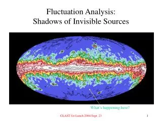
Fluctuation Analysis:Shadows of Invisible Sources What’s happening here? GLAST for Lunch 2004 Sept. 23
The Basic Idea There is background emission between the sources that GLAST will detect. Some of it comes from gas in our galaxy. Some comes from outside our galaxy, and it seems to be isotropic. Its intensity is ~ 10-5 photons/cm2 sec ster (E>100 MeV). It is composed of, partially or in total, of contributions from point sources too faint to detect individually. There’s a trick that allows us to learn something about the flux distribution of these sources. This is taken entirely from Tom Willis’s dissertation (1996). Measure the “diffuse” intensity in pixels of solid angle containing no detectable point sources. If there are N faint sources per steradian, the relative fluctuation in intensity measurements from pixel to pixel is (N)-1/2. It’s not really that simple if the sources are not the same brightness. The number of sources per steradian with flux between S and S+dS is called dN/dS. GLAST for Lunch 2004 Sept. 23
The Hairy Math Part For a given pixel, the total intensity Where K is the number of sources in the pixel. The joint probability distribution of K and the Si is Using this to get the probability distribution of X is a convolution problem, best done with Fourier transforms. The characteristic function Finally the distribution of pixel fluxes is GLAST for Lunch 2004 Sept. 23
Diffuse + Point Sources One question of considerable interest is whether there is a truly diffuse extragalactic background. That will show up as a reduction in the fluctuations, as if there was a huge density of very weak sources. Here’s a simulated result. The three curves represent P(X) for populations with a mixture of point sources and truly diffuse emission: 10%, 50%, and 100% sources. 10% 50% 90% GLAST for Lunch 2004 Sept. 23
How Reality Makes Life Harder • There is always a non-negligible contribution from the Galactic diffuse flux, no matter how far away from the Galactic plane. • Each measurement has a noise contribution from Poisson photon-counting statistics. • It is necessary to choose a pixel size. Large pixels have less Poisson noise, but they can contain so many sources that the fluctuation signal is washed out. The optimum choice depends on the signal you expect to see. • Some theoretical dN/dS choices violate the Olbers’ Paradox constraint: The average “diffuse” intensity is which must not diverge. Smax is the threshold for detecting individual sources. If dN/dS doesn’t cooperate, it’s necessary to put in an infrared cutoff at Smin. In fact, the intensity must be set equal to the observed value. GLAST for Lunch 2004 Sept. 23
EGRET Results (Power Law) Tom Willis applied this method to EGRET data with three different choices of dN/dS. The simplest choice is a truncated power law with Smin = 10-10 photons/cm2 sec. The results aren’t sensitive to Smin if it’s this small. Information from fluctuations is almost orthogonal to the information obtained from the detected sources. In the decade of flux below the EGRET threshold, there are 100-300 point sources, contributing 4-15% of the isotropic background. Constraints from detected sources Constraints from fluctuations Combined constraints GLAST for Lunch 2004 Sept. 23
EGRET Results (Other Models) • The other choices of dN/dS have some physics in them. • Salamon & Stecker (1994) proposed that the gamma ray luminosity of a blazar could be obtained from the radio luminosity by a simple scaling law with two adjustable parameters: • Lr = 10 L (Luminosity scaling) • = (/r)2 (Jet opening angle abundance) The radio dN/dS is a broken power law with slopes of about –1.96 and –0.83. Changing the parameters and modifies the position of the knee and the normalization. Chiang et al. (1995) considered the luminosity function, dN/dL, of blazars, assuming a simple form of luminosity evolution. With a cosmological model this can be translated into dN/dS. They assumed a broken power law shape for dN/dL. From the detected blazars they obtained only a rough constraint for the low-L part of the function (slope = -2.9 2.0). Willis’s fluctuation analysis tightens this to –1.0 > slope > -1.9. GLAST for Lunch 2004 Sept. 23
EGRET Results (Summary) Here’s a summary of the EGRET results. It shows the number of point sources with flux > S at high galactic latitude as a function of S. With GLAST’s detection threshold of about 10-9, it should find something like 1000-10,000 sources. Caveat: This is probably believable only down to about 10-8. Observed blazars GLAST for Lunch 2004 Sept. 23