Download

1 / 16
160 likes | 180 Views
Explore a macroeconomic model of health care production and policy, distinguishing health services from health and analyzing the impact of technology. Learn how goods like non-medical and medical items are valued and produced, and how buying patterns affect health and consumption expenditures. Discover the optimal health share and consider the relationship between health, consumption, and changes in preferences and budgets. Delve into the intersection of macroeconomy and health outcomes, examining the complex relationship between economic factors, stress, drinking behaviors, and health outcomes at individual and societal levels.

E N D
Economics 7550 – Fall 2019 Lecture 2 – A Model of Health Care Production and Policy From Zweifel and Breyer
Purpose • Is there a general way to model (in an aggregate way) health policy? • We would like to distinguish health services from health? • How does technology factor in?
C We produce and value these! C = Home Good H = Health C = C(X) X = Non-medical Good M = Medical Good We buy these! X H M
C C = Home Good H = Health C = C(X), Why? X = Non-medical Good M = Medical Good Why do these look like this? X H Y(H) = pX + qM Y3 Y2 Y1 Y0 Y = pX + qM H = H (M), Why? M
Y = pX + qM Budget Constraint This leads to a relationship between goods X and M. If we differentiate the function, realizing that H = H(M), we get: This leads to:
Normally: If Either equals 0, negative relationship occurs This implies that more M less X. Here, if you buy more M, you’re healthier -- it may allow you to buy more X as well. Thenmore M more X
C C = C(X) X H Y(H) = pX + qM Y = pX + qM H = H (M) M
C We Value These U = U(C, H) C = C(X) X H Y(H) = pX + qM Y = pX + qM H = H (M) M
C U = U(C, H) C = C(X) C* X* X H H* Y(H) = pX + qM Q* Y = pX + qM M* H = H (M) Q* = qM*/y(H*) = Optimal Health Share M
Some Macro thoughts • We may not know much about H or C, but we can measure [qM] and [pX]. • Let H = person-years of good health qM = national health expenditures pX = aggregate consumption expenditures • Suppose there’s an improvement in health technology.
C U = U(C, H) C = C(X) C* X* X H H* Y(H) = pX + qM Q* M* H = H (M) H+ = H+(M) M
Other types of changes • Preferences between health and consumption. • C (X) is not constant. Better education, for example, may increase C. • Budget constraint is subject to changes in p and in q, as well as to increasing incomes (or wage rates). • Institutional factors (e.g. Social Security, Medicare, National Health Insurance) may make a difference.
Ruhm on Macroeconomy and Health • In 1970s there was a lot of literature (Brenner, a sociologist, and others) that said • Bad economy bad health • They did some time series analysis that purported to show that a bad economy had adverse health impacts. • The answer, not surprisingly, is “well, it depends.”
Let’s look at drinking • Bad economy stress ↑ drinking ↑ • BUT, bad economy income drinking . • Drinking less drunk driving and fewer deaths from drunk driving.
These should be examined at the individual level • I looked at this using a 2001 database.
Income and Alcohol The relationship is complicated.