Classification and Prediction
Classification and Prediction. - The Course. DS. OLAP. DP. DW. DS. DM. Association. DS. Classification. Clustering. DS = Data source DW = Data warehouse DM = Data Mining DP = Staging Database. Chapter Objectives. Learn basic techniques for data classification and prediction.


Classification and Prediction
E N D
Presentation Transcript
- The Course DS OLAP DP DW DS DM Association DS Classification Clustering DS = Data source DW = Data warehouse DM = Data Mining DP = Staging Database
Chapter Objectives • Learn basic techniques for data classification and prediction. • Realize the difference between the following classifications of data: • supervised classification • prediction • unsupervised classification
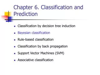
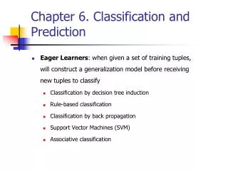
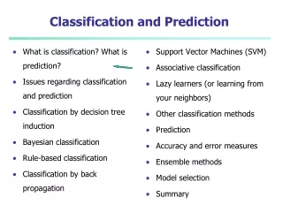
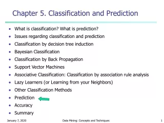
Chapter Outline • What is classification and prediction of data? • How do we classify data by decision tree induction? • What are neural networks and how can they classify? • What is Bayesian classification? • Are there other classification techniques? • How do we predict continuous values?
What is Classification? • The goal of data classification is to organize and categorize data in distinct classes. • A model is first created based on the data distribution. • The model is then used to classify new data. • Given the model, a class can be predicted for new data. • Classification = prediction for discrete and nominal values
What is Prediction? • The goal of prediction is to forecast or deduce the value of an attribute based on values of other attributes. • A model is first created based on the data distribution. • The model is then used to predict future or unknown values • In Data Mining • If forecasting discrete value Classification • If forecasting continuous value Prediction
Supervised and Unsupervised • Supervised Classification = Classification • We know the class labels and the number of classes • Unsupervised Classification = Clustering • We do not know the class labels and may not know the number of classes
Preparing Data Before Classification • Data transformation: • Discretization of continuous data • Normalization to [-1..1] or [0..1] • Data Cleaning: • Smoothing to reduce noise • Relevance Analysis: • Feature selection to eliminate irrelevant attributes
Application • Credit approval • Target marketing • Medical diagnosis • Defective parts identification in manufacturing • Crime zoning • Treatment effectiveness analysis • Etc
Classification is a 3-step process • 1. Model construction (Learning): • Each tuple is assumed to belong to a predefined class, as determined by one of the attributes, called the class label. • The set of all tuples used for construction of the model is called training set. • The model is represented in the following forms: • Classification rules, (IF-THEN statements), • Decision tree • Mathematical formulae
1. Classification Process (Learning) Classification Method Classification Model IF Income = ‘High’ OR Age > 30 THEN Class = ‘Good OR Decision Tree OR Mathematical For Training Data class
Classification is a 3-step process 2. Model Evaluation (Accuracy): • Estimate accuracy rate of the model based on a test set. • The known label of test sample is compared with the classified result from the model. • Accuracy rate is the percentage of test set samples that are correctly classified by the model. • Test set is independent of training set otherwise over-fitting will occur
2. Classification Process (Accuracy Evaluation) Classification Model Accuracy 75% class
Classification is a three-step process 3. Model Use (Classification): • The model is used to classify unseen objects. • Give a class label to a new tuple • Predict the value of an actual attribute
3. Classification Process (Use) Classification Model Good
Classification Methods Classification Method • Decision Tree Induction • Neural Networks • Bayesian Classification • Association-Based Classification • K-Nearest Neighbour • Case-Based Reasoning • Genetic Algorithms • Rough Set Theory • Fuzzy Sets • Etc.
Evaluating Classification Methods • Predictive accuracy • Ability of the model to correctly predict the class label • Speed and scalability • Time to construct the model • Time to use the model • Robustness • Handling noise and missing values • Scalability • Efficiency in large databases (not memory resident data) • Interpretability: • The level of understanding and insight provided by the model
Chapter Outline • What is classification and prediction of data? • How do we classify data by decision tree induction? • What are neural networks and how can they classify? • What is Bayesian classification? • Are there other classification techniques? • How do we predict continuous values?
What is a Decision Tree? • A decision tree is a flow-chart-like tree structure. • Internal node denotes a test on an attribute • Branch represents an outcome of the test • All tuples in branch have the same value for the tested attribute. • Leaf node represents class label or class label distribution
Sample Decision Tree Excellent customers Fair customers 80 Income < 6K >= 6K Age 50 YES No 20 10000 6000 2000 Income
Sample Decision Tree 80 Income <6k >=6k NO Age Age 50 >=50 <50 NO Yes 20 2000 6000 10000 Income
Sample Decision Tree http://www-lmmb.ncifcrf.gov/~toms/paper/primer/latex/index.html http://directory.google.com/Top/Science/Math/Applications/Information_Theory/Papers/
Decision-Tree Classification Methods • The basic top-down decision tree generation approach usually consists of two phases: • Tree construction • At the start, all the training examples are at the root. • Partition examples are recursively based on selected attributes. • Tree pruning • Aiming at removing tree branches that may reflect noise in the training data and lead to errors when classifying test data improve classification accuracy
How to Specify Test Condition? • Depends on attribute types • Nominal • Ordinal • Continuous • Depends on number of ways to split • 2-way split • Multi-way split
CarType Family Luxury Sports CarType CarType {Sports, Luxury} {Family, Luxury} {Family} {Sports} Splitting Based on Nominal Attributes • Multi-way split: Use as many partitions as distinct values. • Binary split: Divides values into two subsets. Need to find optimal partitioning. OR
Size Small Large Medium Size Size Size {Small, Medium} {Small, Large} {Medium, Large} {Medium} {Large} {Small} Splitting Based on Ordinal Attributes • Multi-way split: Use as many partitions as distinct values. • Binary split: Divides values into two subsets. Need to find optimal partitioning. • What about this split? OR
Splitting Based on Continuous Attributes • Different ways of handling • Discretization to form an ordinal categorical attribute • Static – discretize once at the beginning • Dynamic – ranges can be found by equal interval bucketing, equal frequency bucketing (percentiles), or clustering. • Binary Decision: (A < v) or (A v) • consider all possible splits and finds the best cut • can be more compute intensive
Tree Induction • Greedy strategy. • Split the records based on an attribute test that optimizes certain criterion. • Issues • Determine how to split the records • How to specify the attribute test condition? • How to determine the best split? • Determine when to stop splitting
How to determine the Best Split fair customers Good customers Customers Income Age <10k >=10k young old
How to determine the Best Split • Greedy approach: • Nodes with homogeneous class distribution are preferred • Need a measure of node impurity: pure High degree of impurity Low degree of impurity 50% red 50% green 75% red 25% green 100% red 0% green
Measures of Node Impurity • Information gain • Uses Entropy • Gain Ratio • Uses Information Gain and Splitinfo • Gini Index • Used only for binary splits
Algorithm for Decision Tree Induction • Basic algorithm (a greedy algorithm) • Tree is constructed in a top-down recursive divide-and-conquer manner • At start, all the training examples are at the root • Attributes are categorical (if continuous-valued, they are discretized in advance) • Examples are partitioned recursively based on selected attributes • Test attributes are selected on the basis of a heuristic or statistical measure (e.g., information gain) • Conditions for stopping partitioning • All samples for a given node belong to the same class • There are no remaining attributes for further partitioning – majority voting is employed for classifying the leaf • There are no samples left
Classification Algorithms • ID3 • Uses information gain • C4.5 • Uses Gain Ratio • CART • Uses Gini
Entropy: Used by ID3 Entropy(S) = - p log2 p - q log2 q • Entropy measures the impurity of S • S is a set of examples • p is the proportion of positive examples • q is the proportion of negative examples
ID3 pno = 5/14 play pyes = 9/14 don’t play Impurity= - pyes log2 pyes - pno log2 pno = - 9/14 log2 9/14 - 5/14 log2 5/14 = 0.94 bits
ID3 outlook humidity temperature windy sunny overcast rainy high normal hot mild cool false true play 0.98 bits * 7/14 0.92 bits * 6/14 0.81 bits * 4/14 0.81 bits * 8/14 0.0 bits * 4/14 0.97 bits * 5/14 0.59 bits * 7/14 1.0 bits * 4/14 1.0 bits * 6/14 don’t play + = 0.69 bits + = 0.79 bits + = 0.91 bits + = 0.89 bits gain: 0.15 bits gain: 0.03 bits gain: 0.05 bits 0.94 bits maximal information gain amount of information required to specify class of an example given that it reaches node 0.97 bits * 5/14 gain: 0.25 bits
humidity temperature windy high normal hot mild cool false true play 0.0 bits * 3/5 0.0 bits * 2/5 0.92 bits * 3/5 0.0 bits * 2/5 1.0 bits * 2/5 0.0 bits * 1/5 1.0 bits * 2/5 don’t play + = 0.0 bits + = 0.40 bits + = 0.95 bits gain: 0.97 bits gain: 0.57 bits gain: 0.02 bits ID3 outlook sunny overcast rainy 0.97 bits maximal information gain
humidity temperature windy high normal hot mild cool false true play 1.0 bits *2/5 0.92 bits * 3/5 0.0 bits * 3/5 0.92 bits * 3/5 1.0 bits * 2/5 0.0 bits * 2/5 don’t play + = 0.95 bits + = 0.95 bits + = 0.0 bits gain: 0.02 bits gain: 0.02 bits gain: 0.97 bits ID3 outlook overcast sunny rainy 0.97 bits humidity high normal
ID3 play don’t play outlook sunny overcast rainy Yes humidity windy high true false normal Yes No No Yes
C4.5 • Information gain measure is biased towards attributes with a large number of values • C4.5 (a successor of ID3) uses gain ratio to overcome the problem (normalization to information gain) • GainRatio(A) = Gain(A)/SplitInfo(A) • Ex. • gain_ratio(income) = 0.029/0.926 = 0.031 • The attribute with the maximum gain ratio is selected as the splitting attribute
CART • If a data set D contains examples from n classes, gini index, gini(D) is defined as where pj is the relative frequency of class j in D • If a data set D is split on A into two subsets D1 and D2, the gini index gini(D) is defined as • Reduction in Impurity: • The attribute provides the smallest ginisplit(D) (or the largest reduction in impurity) is chosen to split the node (need to enumerate all the possible splitting points for each attribute)
CART • Ex. D has 9 tuples in buys_computer = “yes” and 5 in “no” • Suppose the attribute income partitions D into 10 in D1: {low, medium} and 4 in D2 but gini{medium,high} is 0.30 and thus the best since it is the lowest • All attributes are assumed continuous-valued • May need other tools, e.g., clustering, to get the possible split values • Can be modified for categorical attributes
Comparing Attribute Selection Measures • The three measures, in general, return good results but • Information gain: • biased towards multivalued attributes • Gain ratio: • tends to prefer unbalanced splits in which one partition is much smaller than the others • Gini index: • biased to multivalued attributes • has difficulty when # of classes is large • tends to favor tests that result in equal-sized partitions and purity in both partitions
Other Attribute Selection Measures • CHAID: a popular decision tree algorithm, measure based on χ2 test for independence • C-SEP: performs better than info. gain and gini index in certain cases • G-statistics: has a close approximation to χ2 distribution • MDL (Minimal Description Length) principle (i.e., the simplest solution is preferred): • The best tree as the one that requires the fewest # of bits to both (1) encode the tree, and (2) encode the exceptions to the tree • Multivariate splits (partition based on multiple variable combinations) • CART: finds multivariate splits based on a linear comb. of attrs. • Which attribute selection measure is the best? • Most give good results, none is significantly superior than others
Underfitting and Overfitting Overfitting Underfitting: when model is too simple, both training and test errors are large
Overfitting due to Noise Decision boundary is distorted by noise point
Underfitting due to Insufficient Examples Lack of data points in the lower half of the diagram makes it difficult to predict correctly the class labels of that region - Insufficient number of training records in the region causes the decision tree to predict the test examples using other training records that are irrelevant to the classification task
Two approaches to avoid Overfitting • Prepruning: • Halt tree construction early—do not split a node if this would result in the goodness measure falling below a threshold • Difficult to choose an appropriate threshold • Postpruning: • Remove branches from a “fully grown” tree—get a sequence of progressively pruned trees • Use a set of data different from the training data to decide which is the “best pruned tree”