Download
1 / 31
370 likes | 720 Views
Uncertainty Most intelligent systems have some degree of uncertainty associated with them. The types of uncertainty that can occur in KBS may be caused by problems with the data. 1. Data might be missing or unavailable.

E N D
Uncertainty • Most intelligent systems have some degree of uncertainty associated with them. • The types of uncertainty that can occur in KBS may be caused by problems with the data. • 1. Data might be missing or unavailable. • 2. Data might be present but unreliable or ambiguous due to measurement errors, multiple conflicting measurements etc. • 3. The representation of the data may be imprecise or inconsistent. • 4. Data may just be user's best guess. • 5. Data may be based on defaults and the defaults may have exceptions.
Alternatively, the uncertainty may be caused by the represented knowledge since • it might represent best guesses of the expert that are based on plausible or statistical observations • it might not be appropriate in all situations • Given these numerous sources of errors, the most KBS requires the incorporation of some form of uncertainty management. • While implementing some uncertainty scheme, we must be concerned with three issues. • 1. How to represent uncertain data. • 2. How to combine two or more pieces of uncertain data. • 3. How to draw inference using uncertain data. • Several methods have been proposed for handling uncertain information.
Probabilities (Oldest with strong mathematical basis) • The chance that a particular event will occur is equal to the number of ways the event can occur divided by the total number of all possible events. • Example: The probability of throwing two successive heads with a fair coin is 0.25 • * Total of four possible outcomes are : • H-H, H-T, T-H & T-T • * Since there is only one way of getting H-H, • the probability = ¼ = 0.25 • Probability is a way of turning opinion or expectation into numbers. It is a number between 0 to 1 that reflects the likelihood of an event.
An impossible event has a probability of 0 while a certain event has a probability. • We write P(A) for the probability of an event A. • A set of independent events, call it sample space may represent all possible outcomes. It is the set of all possible outcomes of a random experiment. • The possibility of all events S = {A1, A2, …, An} must sum up to certainty i.e. P(A1) + ---- + P(An) = 1 • Event: Every non-empty subset A (of sample space S) is called an event. • null set is an impossible event. • S is a sure event • Since the events are the set, it is clear that all set operations can be performed on the events.
1. A B is an event "both A and B". 2. A B is an event "either A or B or both" 3. A' is an event "not A" 4. A - B is an event "A but not B 5. Events A and B are mutually exclusive, if A B= Axioms of Probability : Let S be a sample space, A and B are events. 1. P(A) 0 2. P(S) = 1 3. P(A’ ) = 1 - P(A) 4. P(A B) = P(A) + P(B), if events A and B are utually exclusive 5. P(A B) = P(A) + P(B) – P(A B) Proof: A B= A (A’ B) Therefore, P(A B)= P(A (A’ B)) = P(A) + P(A’ B) = P(A) + P(A’ B) + P(A B) - P(A B) = P(A) + P(B)- P(A B)
In general, for mutually exclusive events A1, …, An in S • P(A1 A2… An ) = P(A1) + P(A2) + …+ P(An) • Joint Probability of the occurrence of two event (which are independent ) is written as P (A and B) is defined by P(A and B) = P(A) * P(B) • Example: We toss two fair coins separately. • Let • P(A) = 0.5 , Probability of getting Head of first coin • P(B) = 0.5, Probability of getting Head of second coin • Probability of getting Heads on both the coins is Joint probability • = P(A and B) • = P(A) * P(B) = 0.5 X 0.5 = 0.25 • The probability of getting Heads on one or both of the coins i.e. the union of the probabilities P(A) and P(B) is expressed as • P(A or B) = P(A) + P(B) - P(A) * P(B) • = 0.5 X 0.5 - 0.25 • = 0.75
Conditional Probability : It relates the probability of one event to the occurrence of another i.e. probability of the occurrence of an event E given that an event F is known to have occurred. • Probability of an event E, given the occurrence of an event F is denoted by P(E | F) and is defined as follows: Number of events favourable to F which are also favourable to E • P(E | F) = • No. of events favourable to F • = P(E and F) / P(F)
Example: What is the probability of a person to be male if person chosen at random is 80 years old and if the following are given • Any person chosen at random being male is about 0.50 • Let the probability of a given person be 80 years old chosen at random is equal to 0.005 • Let the probability that a given person chosen at random is both male and 80 years old may be =0.002 • Then the probability that an 80 years old person chosen at random is male is calculated as follows: • P(X is male | Age of X is 80) • = [P(X is male and the age of X is 80)] / [P(Age of X is 80)] • = 0.002 / 0.005 = 0.4
Result : If the events E and F defined on the sample space S of a random experiments are independent then • P(E | F) = P(E) • Proof: P(E | F) = P(E and F) / P(F) • = P(E) * P(F) / P(F) • = P(E) • Similarly, P(F | E) = P(F) • Bayesian Probabilities • This approach relies on the concept that one should incorporate the prior probability of an event into the interpretation of a situation. • Bayes theorem provides a mathematical model for this type of reasoning where prior beliefs are combined with evidence to get estimates of uncertainty. • Bayes theorem relates the conditional probabilities of events i.e. it allows us to express the probability P(A | B) in terms of the probabilities of P(B | A), P(A) and P(B).
This is often important since if P(B | A), P(A) and P(B) are given then one can compute probability P(A | B) as follows: • P(A | B) = [P(B | A) * P(A) ] / P(B) • Proof: • P(A | B) = P(A and B) / P(B) • P(B | A) = P(B and A) / P(A) • Therefore, P(A | B) = [P(B | A) * P(A) ] / P(B) • Here B represents evidence and A represents the set of hypotheses. • Some Expert Systems use Bayesian theory to derive further concepts. • Example • i. If _then rule in rule-based Systems • if X is true then Y can be concluded with probability P • i.e. • IF the patient has a cold THEN the patient will sneeze (0.75)
But if we reason abductively and observe that the patient sneezes while knowing nothing about whether the patient has a cold or not, then what can we conclude about it? • To make this more concrete, consider the following example: • Example: Find whether Bob has a cold (hypotheses) given that he sneezes (the evidence) i.e., calculate P(H | E). Suppose that we know in general • P(H) = P (Bob has a cold) = 0.2 • P(E | H)= P(Bob was observed sneezing | Bob has a cold) = 0.75 • P(E | ~H)= P(Bob was observed sneezing | Bob does not have a cold) = 0.2 • Now • P(H | E) = P(Rob has a cold | Rob was observed sneezing) • = [ P(E | H) * P(H) ] / P(E)
We can compute P(E) as follows: • P(E) = P(E | H) * P(H) + P(E | ~H) * P(~H) • = (0.75)(0.2) + (0.2) (0.8) = 0.31 • Hence • P(H | E) = [(0.75 * 0.2)] / 0.31 = 0.48387 • We can conclude that “Rob’s probability of having a cold given that he sneezes” is about 0.5 • We can also determine what is his probability of having a cold if he was not sneezing • P(H | ~E) = [P(~E | H) * P(H)] / P(~E) • = [(1 – 0.75) * 0.2] / (1 – 0.31) • = 0.05 / 0.69 • = 0.072 • Hence “Rob’s probability of having a cold if he was not sneezing” is 0.072
Result: Show that P(E) = P(E | H) * P(H) + P(E | ~H) * P(~H) Proof: P(E) = P( E and H) + P( E and ~H) We know that P( E and H) = P(E | H) * P(H) P( E and ~H) = P(E | ~H) * P(~H) Therefore, P(E) = P( E | H) * P(H) + P( E | ~H) * P(~H)
Advantages and disadvantages of Bayesian Method • Advantages: • They have sound theoretical foundation in probability theory and thus are currently the most mature of all certainty reasoning methods. • Also they have well-defined semantics for decision making. • Disadvantages: • They require a significant amount of probability data to construct a KB. • - For example, a diagnostic system having 50 detectable conclusions (R) and 300 relevant and observable characteristics (S) requires a minimum of 15,050 (R*S + R) probability values assuming that all of the conclusions are mutually exclusive.
If conditional probabilities are based on statistical data, the sample sizes must be sufficient so that the probabilities obtained are accurate. • If based on human experts, then question of values being consistent & comprehensive arise. • The reduction of the associations between the hypothesis and evidence to numbers also eliminates the knowledge embedded within. • The associations that would enable the system to explain its reasoning to a user are lost and also the ability to browse through the hierarchy of evidences to hypothesis.
Probabilities in Rules and Facts of Production System • We normally assume that the facts are always completely true but facts might also be probably true. • Probability can be put as the last argument to a predicate representing fact. • For example, a fact "battery in a randomly picked car is 4% of the time dead" in Prolog is expressed as battery_dead (0.04). • This fact indicates that battery is dead is sure with probability 0.04. • Similarly probabilities can also be added to rules.
Examples: Consider the following probable rules and their corresponding Prolog representation. • "if 30% of the time when car does not start, it is true that the battery is dead " • battery_dead (0.3) :- ignition_not_start(1.0). • Here 30% is rule probability. If right hand side of the rule is certain, then we can even write above rule as: battery_dead(0.3) :- ignition_not_start. • "the battery is dead with same probability that the voltmeter is outside the normal range" • battery_dead(P) :-voltmeter_measurment_abnormal(P). • If we want to ignore very weak evidences for conclusion to avoid unnecessary computation, then we can rewrite above rule as: • battery_dead(P) :- voltmeter_measurment_abnormal(P), P > 0.1.
Cumulative Probabilities • When we want to reason about whether the battery is dead, we should gather all relevant rules and facts. • Combining probabilities from facts and successful rules to get a cumulative probability of the battery being dead is an important issue. • According to Bayesian approach based on formal probability theory for uncertainty, there are two issues. • - First issue is that the probability of a rule to succeed depends on probabilities of sub goals on the right side of a rule. • * The cumulative probability of conclusion can be calculated by using and-combination.
* In this case, probabilities of sub goals in the right side of rule are multiplied, assuming all the events are independent of each other using the formula • Prob(A and B and C and .....) = • Prob(A) * Prob(B) * Prob(C) * ... • - Second issue is that the rules with same conclusion can be uncertain for different reasons. • * So when we have more than one rules with the same predicate name, say, 'p' having different probabilities, then in order to get cumulative likelihood of 'p', we have to use or-combination to get overall probability of predicate 'p'. • The following formula is used to get 'or' probability if events are mutually independent. • Prob(A or B or C or ...) • = 1 - [(1 - Prob(A)) (1 - Prob(B)) (1 - Prob(C))....]
Examples: 1. "half of the time when a car has an electrical problem, then the battery is dead" battery_dead(P):-electrical_prob(P1), P is P1*0.5. Here 0.5 is a rule probability. 2. "95% of the time when a car has electrical problem and battery is old, then the battery is dead" battery_dead(P) :- electrical_prob(P1), battery_old(P2), P is P1 * P2 * 0.95. 3. Find the probability of battery being dead if probability of electric problem is 0.6 and that of battery old is 0.9 using rule defined in above example. Solution: Given P1 = 0.6 and P2 = 0.9 Then P = P1 * P2 * 0.95 = 0.513 Therefore, the probability of battery being dead is 0.513 if probability of electric problem is 0.6 and that of battery dead is 0.9
Computing Cumulative Probabilities using Prolog: • We have to assumes that the sub goals and rules are independent of each other. • And-combination: collect all the probabilities in a list and compute the product of these to get and-combination effect. • and_combination([P], P). • and_combination([H | T], P) :- and_combination(T, P1), P is P1 * H. • Examples: • 1. " when a car has electrical problem and battery is old then the battery is dead" • battery_dead(P) :- electrical_prob(P1), battery_old(P2), • and_combination([P1, P2], P).
2. "95% of the time when a car has electrical problem and battery is old then the battery is dead". • Here the rule probability (0.95) is also include in and combination. • battery_dead(P) :- electrical_prob(P1), battery_old(P2), • and_combination([P1, P2, 0.95], P). • The rule probability can be thought of hidden and is “and' combined along with associated probabilities in the rule. • Example: Suppose we have the following program containing rules and facts • find(P) :- first(P1), second(P2), third, • and_combination([P1, P2, 0.7], P). • first(0.5). • second(0.75). • third. • ?- find(P). Ans: P = 0.2625
Or-combination: Get all the probabilities of the same predicate name defined as head of different rules in a list and compute or_combination probability using the following formula. • Prob(A or B or C or ...) = 1 - [(1 - Prob(A)) (1 - Prob(B)) (1 - Prob(C))....] • or_combination([P], P). • or_combination([H|T],P) :- or_combination(T, P1), • P is 1 -((1 - H) * (1 - P1)). • Examples: • 1. Consider the following rules and facts. • get(0.6) :- first. • get(0.8) :- second, third. • get(0.5) :- first, fourth. • We can define another predicate for computing overall probability or likelihood of 'get' using or_combination.
overall_get (P) :- findall(P1, get(P1), L), or_combination(L, P). ?- overall_get(P) Ans: P = 0.960 2. Consider rules with and-combination as follows: get(0.6) :- first. get(0.8) :- second. get(P) :- third(P1), fourth(P2), and_combination([P1, P2, 0.8], P). first. second. third(0.5), fourth(0.6). overall_get(P) :- findall(P1, get(P1), L), or_combination(L, P). ?- overall_get(P). ?- findall(P1, get(P1), L), or_combination(L, P) Ans: L = [0.6, 0.8, 0.24] P = 0.9392
Handling Negative Probabilities • Sub goals in rules which are not true sometimes cause problems for probabilities. Consider the following example. • Example: Consider a rule • g(P) :- a(P1), b(P2), not(c(P3)). • - Here a, b and c are all uncertain and if the rule itself has a certainty factor of 0.8, then cumulative probability P can not be calculated by simply using • and_combination([P1, P2, P3, 0.8], P) because if there is any evidence for c, the rule will fail always. • The way to handle this is that the probability of something being false is (1 - probability of it being true). • Therefore, the rule is rewritten as • g(P) :- a(P1), b(P2), not(c(P3)), inverse(P3, P4), • and_combination([P1, P2, P4, 0.8], P). • inverse(P, Q) :- Q is 1 - P. • So we should not use probabilities specified in sub goals having 'not' but use inverse probabilities in calculating cumulative probabilities.
Production System for Diagnosis of malfunctioning Equipment using Probability • Let us develop production system for diagnosis of malfunctioning of television using probabilities. • We have to identify situations when television is not working properly. We broadly imagine one of two things may be improperly adjusted. • - the controls (knobs and switches) • - the receiver (antenna or cable) • Let us estimate probabilities of these two things. • Knobs adjustment: • Knobs might be adjusted wrong on television because of the following reasons (by no mean exhaustive) • 1. If television is old and require frequent adjustment. • 2. Unusual usage (i.e., any thing strange has happened lately that required adjustment of the knobs). • 3. If children use your set and they play with the knobs.
Let us write the following rules: • 1. Rule for frequent adjustment • "If a set requires frequent readjustment, then it is quite reasonable that the set is maladjusted today". • Assume that this rule is 50% sure. • In Prolog it is coded as: • maladjusted(0.5) :- askif(freq_adjustment_needed). • Here askif predicate types out a question for the user and checks if the response is positive or negative. • 2. Rule for unusual usage of the system • "let us say that it is 40% to be reasonable that the set is maladjusted today because of unusual usage". • maladjusted(0.4) :- askif( recent_unusual_usage).
3. Rule for children usage • "If children are present and use your set and they play with the knobs with some probability, then it is 90% sure that set is maladjusted today". • maladjusted(P):-askif(children_present, P1), • askif(children_twidle_knobs, P2), • and_combine([P1, P2, 0.9], P). • This rule says that when both the conditions hold (children are present and children twiddle with knobs) with some probabilities, then it means, "it is 90% sure that set is maladjusted today". • Finally, to get the cumulative probability for the set was adjusted recently, we need to combine probabilities of all the rules using or-combination explained earlier.
The corresponding rule is: • recently_adjusted(P) :-findall(X, maladjusted(C), L), or_combine(L, P). • The rule for diagnosis which we assume to be 80% sure might be: • diagnosis('Knobs on the set required adjustment', P) :- recently_adjusted(P1), askif(operation(abnormal)), and_combine([P1, 0.8], P). • Alternatively, if there is some uncertainty about whether the system behaviour is normal, then we could include a probability as another argument in operation predicate as: • diagnosis('Knobs on the set required adjustment', P) :- recently_adjusted(P1), • askif (operation(abnormal, P2)), • and_combine([P1, P2, 0.8], P).
We must note that these rules are to be carefully designed in consultation with domain expert. • Let us consider other kinds of television diagnosis such as antenna or cable connection etc. • source_prob(0.8) :- askif(television_old). • source_prob(0.95) :- askif(antenna_old). • source_prob(0.98) :- askif(cable_old). • source_prob(0.3) :- askif(recent_furniture_rearranging). • overall_source_pr(P):-findall(X,source_prob(X), L), or_combine(L, P). • Following are two rules for such diagnosis. • diagnosis( 'Antenna connection faulty', P) :- askif(source_type_antenna), • askif(operation(abnormal)), • overall_source_prob(P).
diagnosis( 'Cable connection faulty', P) :- askif(source_type_cable), • askif(operation(abnormal)), • overall_source_prob(P). • To run such a system, put a Goal as: • ?- diagnosis(D, P). • Each answer to the above Goal will bind D to the string representing diagnosis and P to the corresponding probability.