Download
1 / 27
270 likes | 358 Views
This study explores the spatial prediction of coho salmon counts on stream networks in Oregon using Geostatistical methods. It includes data analysis, latent process modeling, model estimation, cross-validation, and simulation studies. The findings help in understanding and predicting coho salmon populations.

E N D
Spatial Prediction of Coho Salmon Counts on Stream Networks Dan Dalthorp Lisa Madsen Oregon State University September 8, 2005
Sponsors • U.S. EPA STAR grant # CR-829095 • U.S. EPA Program for Cooperative Research on Aquatic • Indicators at Oregon State University grant # CR-83168201-0.
Outline • Introduction (i) Coho salmon data (ii) GEEs for spatial data • Latent process model for spatially correlated counts • Estimation and results • Cross-validation • Simulation study • Conclusions and future research
Coho Salmon Data • Adult Coho salmon counts at selected points in Oregon coastal • stream networks for 1998 through 2003. • Euclidean distance between sampled points. • Stream distance between sampled points.
GEEs for Spatially Correlated Data • Liang and Zeger’s (1986) pioneering paper in Biometrika • introduced GEEs for longitudinal data. • Zeger (1988) developed GEE analysis for a time series of counts • using a latent process model. • McShane, Albert, and Palmatier (1997) adapted Zeger’s model and • analysis to spatially correlated count data. • Gotway and Stroup (1997) used GEEs to model and predict spatially • correlated binary and count data. • Lin and Clayton (2005) develop asymptotic theory for GEE estimators • of parameters in a spatially correlated logistic regression model
The LatentProcess Model Suppose: The latent process allows for overdispersion and spatial correlation in .
The Marginal Model These assumptions imply: For now, we assume a simple constant-mean model and a one-parameter exponential correlation function:
Estimating the Model Parameters To estimate parameters solve estimating equations: where
Iterative Modified Scoring Algorithm Step 0: Calculate initial estimates Step 1: Update .
Step 2: Update . Step 3: Update . Iterate steps 1, 2, and 3 until convergence.
Year Sample Mean Euclidean Distance Stream Distance 1998 6.2451 6.0 6.4941 1999 9.0025 8.7286 9.0765 2000 11.92 10.898 11.481 2001 31.359 31.597 34.541 2002 46.494 46.782 46.725 2003 44.453 41.005 41.829 Assessing Model Fit–Estimatingthe Mean
Year Sample Std. Dev. Euclidean Distance Stream Distance 1998 222.07 221.59 221.59 1999 443.65 442.61 442.54 2000 384.59 384.75 383.90 2001 2508.6 2502.3 2512.3 2002 9286.6 9265.4 9265.4 2003 3650.2 3653.4 3648.4 Assessing Model Fit – Estimating the Variance
Assessing Model Fit – Estimating the Range (Euclidean Distance)
Assessing Model Fit – Estimating the Range (Stream Distance)
Cross validation to compare predictions based on three different assumptions about the underlying spatial process: 1. Null model (spatial independence) : 2. Spatial correlation as a function of Euclidean distance (ed): 3. Spatial correlation as a function of stream network distance (id)
Covariance model _ EuclideanStream distance 1998 -0.001 -0.047 1999 0.007 -0.037 2000 0.013 0.011 2001 -0.005 -0.005 2002 -0.008 -0.007 2003 -0.002 0.020 1. Bias? Not an issue... 2. Precision? Covariance model _ NullEuclideanStream distance 1998 14.7213.25 14.00 1999 20.58 19.7521.17 2000 20.05 19.83 19.74 2001 48.6934.38 37.75 2002 98.5397.04 97.35 2003 60.49 60.92 58.61
Variances of predicteds Null Euclidean Stream 0.04 10.32 4.95 0.05 12.07 7.68 0.04 11.46 6.40 0.13 38.08 33.36 0.22 15.74 10.65 0.14 24.34 25.99 Odds(|Eed| < |Eid|) Year Odds 1998 256:152 1999 267:132 2000 266:171 2001 197:198 2002 266:171 2003 222:197 Total 1474:1021
Simulations For each year, 8 scenarios that mimic the sample means, variances, and ranges from the data were simulated. Mean and variance constant 1. Euclideanspatial correlation 2. Stream network spatial correlation Mean varies randomly by stream network; variance = 3.66 m 1.741 3.Euclideanspatial correlation; long range 4.Euclideanspatial correlation; medium range 5.Euclideanspatial correlation; short range 6.Stream networkspatial correlation; long range 7.Stream networkspatial correlation; medium range 8.Stream networkspatial correlation; short range
Simulation proceedure 1. Simulate vector Z of correlated lognormal-Poissons to cover all sampling sites (n≈ 400) 2. Estimate parameters (m, s2, range) via latent process regression from simulated data for a subset of the sampling sites (blue) 3. Predict Z at the remaining sites (red, m ≈ 400) using: (Gotway and Stroup 1997) 4. Repeat 100 times for each scenario (8) and year (6)
Use Euclidean distance or stream distance in covariance model? Evaluation of predictions via two measures: where:
Summary of Findings Cross-validations: 1. MSPEs same for Euclidean distance and stream network distance; 2. Errors usually smaller with Euclidean distance; 3. Population spikes more likely to be detected with Euclidean distance. Simulations: 1. Euclidean spatial process: Euclidean covariance gives smaller MSPE than does stream network distance covariance; 2. Stream network process: Euclidean covariance model MSPEs comparable to those of stream distance model EXCEPT when network means varied and range of correlation was large.
Future work • -- Incorporate covariates (with some misaligned data); • -- Incorporate downstream distances/flow ratios; • -- Spatio-temporal modeling; • -- Rank correlations in place of covariances; • -- Model selection; • -- Non-random data;