Download
1 / 33
330 likes | 395 Views
Explore the application of Polynomial Regression on agricultural crop yields and apartment rental prices using multiple regression models. Learn how to interpret the results of polynomial regression to predict yields and rental values accurately.

E N D
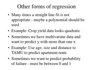
Other forms of regression • Many times a straight line fit is not appropriate - maybe a polynomial should be used • Example: Crop yield data looks quadratic • Sometimes we have multivariate data and want to predict y with more than one x • Example: Use age, size and distance to TAMU to predict apartment rents • Sometimes we want to predict probability of failure - must be between 0 and 1
Polynomial Regression • Example: Crop Yields • Scatter plot shows curvature - possibly quadratic. • y = b0 + b1x + b2x2 + e • Use sample to estimate the b’s this relationship. • This would be polynomial regression.
Polynomial Regression: Yields Source | SS df MS Number of obs = 16 ---------+------------------------------ F( 2, 13) = 25.19 Model | 2086569.42 2 1043284.71 Prob > F = 0.0000 Residual | 538481.521 13 41421.6554 R-squared = 0.7949 ---------+------------------------------ Adj R-squared = 0.7633 Total | 2625050.94 15 175003.396 Root MSE = 203.52 ------------------------------------------------------------------------------ Yield | Coef. Std. Err. t P>|t| [95% Conf. Interval] ---------+-------------------------------------------------------------------- Date | 293.5805 42.10316 6.973 0.000 202.6221 384.5388 DateSqrd | -4.536984 .6732241 -6.739 0.000 -5.991396 -3.082571 _cons | -1072.373 616.1627 -1.740 0.105 -2403.511 258.7659 ------------------------------------------------------------------------------ • Sample line: y = -1072.373 + 293.5805 x - 4.536984 x2 + e • This equation explains 76% of variability in yields (adjusted R2) • SD of errors is 203.52 (RMSE) • If the 4 conditions are met, we have CI’s for the coefficients • If the 4 conditions are met, we can form CI’s and PI’s for y at a given x
Polynomial Regression: Yields • Residual and normal quantile plots have the same interpretation • Residuals are centered at zero, have equal SD • Residuals are also normal • We can perform inference! • We have CI’s for coefficients of equation - they are valid
y = b0 + b1x + b2x2 +e 95% CI’s for b’s b0 in (-2403, 258) b1 in (202,384) b2 in (-6,-3) Result from calculus - max achieved at x = -b1 /(2 b2) Thus, to maximize yields, we should harvest on day 32 We could form CI’s for mean yield for particular days Could also form PI’s for an individual yield on a particular day Polynomial Regression: Yields
Multiple Regression: BCS Rent • Based on data collected by my class in spring 1999 • Simple random sample of BCS apartment complexes • Want to know which factors (distance to TAMU, age of complex, sq. ft. floor space) affects the monthly rent of two bedroom apartments • Rent = f(distance, age, space) + e • What’s f()?
Multiple Regression: BCS Rent Source | SS df MS Number of obs = 19 ---------+------------------------------ F( 3, 15) = 18.94 Model | 198161.15 3 66053.7166 Prob > F = 0.0000 Residual | 52323.4818 15 3488.23212 R-squared = 0.7911 ---------+------------------------------ Adj R-squared = 0.7493 Total | 250484.632 18 13915.8129 Root MSE = 59.061 ------------------------------------------------------------------------------ Rent | Coef. Std. Err. t P>|t| [95% Conf. Interval] ---------+-------------------------------------------------------------------- Age | -6.654856 2.071647 -3.212 0.006 -11.07047 -2.239245 Dist | -23.27366 11.47989 -2.027 0.061 -47.74247 1.195149 Size | .4828364 .0976556 4.944 0.000 .2746885 .6909843 _cons | 366.9301 111.6425 3.287 0.005 128.9698 604.8904 ------------------------------------------------------------------------------ • Rent ($) = 366 - 6.65 Age (yrs) - 23.27 Distance (mi) + .482 Size (sq. ft) + errors • This equation explains 74% of the variation of rents in Bryan-College Station • The standard deviation of the errors is $59.06. • CI’s indicate that age and distance may not be important factors in rent • Let’s check the conditions before jumping to conclusions
Multiple Regression: BCS Rent • Residual plot indicates curvature - we must have missed a curvature factor. • Look for it - after examination we determined that it was age. • Add a term for age squared - try again.
Multiple Regression: BCS Rent • Rent = b0 + b1 size + b2 dist + b3 age + b4 age2 + e • We tried this equation • Residuals were centered at zero and evenly spread • Adjusted R2 = .8177, Previously .7493 • RMSE = 50.37, Previously 59.03 • Everything’s better! • Let’s check our table
Multiple Regression: BCS Rent • Residuals are centered at zero - evenly spread throughout. • Residuals are also normal. • We can perform inference!
Multiple Regression: BCS Rent Source | SS df MS Number of obs = 19 ---------+------------------------------ F( 4, 14) = 21.18 Model | 214964.171 4 53741.0428 Prob > F = 0.0000 Residual | 35520.4603 14 2537.17574 R-squared = 0.8582 ---------+------------------------------ Adj R-squared = 0.8177 Total | 250484.632 18 13915.8129 Root MSE = 50.37 ------------------------------------------------------------------------------ Rent | Coef. Std. Err. t P>|t| [95% Conf. Interval] ---------+-------------------------------------------------------------------- Distance | -18.82174 9.942284 -1.893 0.079 -40.14581 2.502341 Size | .5293884 .0852274 6.211 0.000 .3465939 .7121829 Age | -22.19967 6.29351 -3.527 0.003 -35.69791 -8.701434 AgeSqrd | .3980626 .1546796 2.573 0.022 .0663079 .7298172 _cons | 449.9577 100.5319 4.476 0.001 234.3383 665.5771 ------------------------------------------------------------------------------ • Rent = 449 - 18.82 Distance + .529 Size - 22.19 Age + .398 Age2 + errors • Based on CI’s - distance may be inconsequential • Likely due to confounding between distance and age (Northgate - close & old) • Could form CI’s for mean rent given (distance, size, age) - beyond scope of course • Could for PI’s for individual rent given (distance, size, age) - beyond scope of course • Only valid for apartments in ranges observed: 300 year old apartment would be very expensive
Logistic Regression • Sometimes we wish to predict the probability of failure (or success) • Example: predict the probability of failure (P) of some system in certain conditions (x) • P(x) = e b0+b1x/(1+e b0+b1x) + e • Given sample data - we will fit it to estimate the probability of failure • Based on a different type of theory - we will not discuss the theory in this course - just applications
Logistic Regression O-rings join sections of the rockets together. There are two joints on each of the two rockets. At each joint there are two O-rings - the primary O-ring and a back-up O-ring. We will use data from NASA (for launches previous to the Challenger explosion) to predict the probability of one O-ring failure. There are a total of 8 O-rings on each shuttle launch.
After each shuttle launch NASA would collect remnants of the launch apparatus from the ocean Examine O-rings for signs of failure There were 4 O-rings each with a back-up O-ring for a total of 8 O-rings The corporation that made the O-rings warned NASA that the performance of the O-rings was highly dependent on temp NASA didn’t have a statistician - even though they collected data Logistic Regression: Shuttle
list Temp Failures Orings Pfail in 1/24 Temp Failures Orings Pfail 1. 53 3 8 .375 2. 56 1 8 .125 3. 57 1 8 .125 4. 63 1 8 .125 5. 66 0 8 0 6. 67 0 8 0 7. 67 0 8 0 8. 67 0 8 0 9. 68 0 8 0 10. 69 0 8 0 11. 70 1 8 .125 12. 70 1 8 .125 13. 70 0 8 0 14. 70 0 8 0 15. 73 0 8 0 16. 74 0 8 0 17. 75 2 8 .25 18. 75 0 8 0 19. 76 0 8 0 20. 76 0 8 0 21. 77 0 8 0 22. 79 0 8 0 23. 81 0 8 0 24. 82 0 8 0 These are the data (from before the disaster) Resulting Equation: P(t) = e 15-.23t/(1+e 15-.23t) Lowest temp = 53 T = 31 on day of disaster P(31) = .9996 (doomed) Now NASA has statisticians Logistic Regression: Shuttle
Notes on Extrapolation • Regression results are only guaranteed to hold in the range of observed data • This doesn’t mean the equation is invalid outside the range • If the same mechanisms drive the phenomena outside the range, then regression is a good predictor • Sometimes - like forecasting - using regression outside the data range is the only way • Exercise caution and common sense with regression outside the data range
Shuttle Question • Even though extrapolation is not guaranteed outside the data range - give it a try - it may provide insight (with the necessary disclaimers) • With the ease of computing - the shuttle disaster should not have happened, a statistician would have predicted a 99.96% probability of failure for the O-rings!
Palm Beach County Analysis • It was pointed out earlier that the scatterplot of Florida counties Buchanan vote versus Total Vote showed heteroscedasticity (unequal SD - “spread out” as you move right) • This can be “fixed” by looking at the logs of the votes instead of the actual vote tallies
Palm Beach County Analysis • To the left - actual vote counts -notice the heteroscedasticity - the SD is not equal throughout • To the right - log of vote counts - the SD is equal throughout - Palm Beach is still an outlier
Palm Beach County Analysis • Errors are normal with mean zero and equal SD • Independence? Do neighboring counties affect each other? • Palm Beach had 432,286 votes • ln(432,286) = 12.97 • PB log(Buchanan) = 8.13 • 99% PI = (5.43,7.79) • In actual votes - PB had about 993 more votes for Buchanan than upper limit of PI
Notes on Statistical Analysis • The statistics show that if the rest of Florida can be used to predict Palm Beach County, then there were an unusually high number of votes for Buchanan in that county. • Statistics do not reveal the cause.
Review of Today’s Topics • Polynomial Regression explains curvature in y as a function of x • Multiple Regression explains y with several x’s • Both of the above depend on normal, mean zero, equal SD, independent errors • Logistic regression predicts the probability of failure (or success) - does not use normal theory