Other Regression
Other Regression. Stuff you might come across. Outline. Generalized Linear Models Logistic regression and Related Survival analysis Generalized Additive Models Time series Quantile regression Polynomial Regression Multilevel modeling Multiple outcome (Multivariate) regression Summary.

Other Regression
E N D
Presentation Transcript
Other Regression Stuff you might come across
Outline • Generalized Linear Models • Logistic regression and Related • Survival analysis • Generalized Additive Models • Time series • Quantile regression • Polynomial Regression • Multilevel modeling • Multiple outcome (Multivariate) regression • Summary
Why Logistic Regression? • Oftentimes the theoretical question involves an aspect of human behavior that can in some way be categorized • It is one thing to use a t-test (or multivariate counterpart) to say groups are different, however it may be the research goal to predict group membership • Clinical/Medical context • Schizophrenic or not • Clinical depression or not • Cancer or not • Social/Cognitive context • Vote yes or no • Preference A over B • Graduate or not • While typically used for dichotomous outcomes (binomial logistic regression), it can be extended to a polytomous one (multinomial logistic regression) • The question of whether to use a categorical variable as predictor or dependent variable is often arbitrary outside of theory, though in some cases the implied causal flow or other considerations would suggest one or the other • In the examples above, we could easily turn them into t-test type analyses comparing e.g. those who voted one way vs. the other • However, it would not make theoretical (causal) sense to suggest that personality traits predict gender, though the computer program won’t stop you
X1 X2 Categorical Y X3 X4 Basic Model (Same as MR)
Logistic Regression • Why not just use regular regression? • With normal regression with continuous outcome we predicted the expected value of Y (i.e. its mean) given a specific value of X • E(Yi|X=xi) • In the population, the conditional average is just the proportion of those who score a ‘1’, and yet even though our range is [0,1], predicted values from an OLS approach would fall outside of that range • Furthermore, if we tried to fit a regular regression assumptions for it would be untenable • We could constrain our outcomes to not go beyond the range but this still would be unsatisfactory
Logistic Regression • A cumulative probability distribution satisfies the 0,1 range problem, so if we can map our linear combination of predictors to something like this and think in terms of predicted probabilities, we can have our linear cake and eat it too • This is essentially what is going on in logistic regression • You may also come across a ‘probit’ model instead of a logit model, that is one that uses the cumulative normal distribution as its basis • They are largely indistinguishable in practice, though the logistic is computationally more easy and its ‘log odds’ interpretation more clear
Logistic Regression • We have all the same concerns here though logistic regression has fewer restrictive assumptions • The only “real” limitation with logistic regression is that the outcome must be nominal • Ratio of cases to variables: using discrete variables requires that there are enough responses in every given category to allow for reasonable estimation of parameters/predictive power • Due to the maximum likelihood approach, some suggest even 50 cases per predictor as a rule of thumb • Also, the greater discrepancy among groups, the less likely the analysis will improve notably over guessing • If you had a 9:1 ratio, one could just guess the majority category and be correct the vast majority of the time • Linearity in the logit – the predictors should have a linear relationship with the logit form of the DV • There is no assumption about the predictors being linearly related to each other • Absence of collinearity among predictors • No outliers • Independence of errors • Assumes categories are mutually exclusive
Model fit • Significance Test: Log-Likelihood (LL) 2 test between Model (M) with predictors + intercept, vs. Intercept (I) only model. • If Likelihood 2 test is significant, the model with additional predictors is best. • Goodness-of-fit statistics help you to determine whether the model adequately describes the data • Hosmer-Lemeshow • Here statistical significance is not desired, and as such it is more of a badness of fit really, and problematic since one can’t accept the null due to non-significance • Best used descriptively perhaps • Pseudo r-squared statistics • In this dichotomous situation we will have trouble with devising an R2 • AIC, BIC • Deviance • Analogous to residual sums of squares from OLS, it is given in comparison to a perfectly fit null model
Coefficients • In interpreting coefficients we’re now thinking about a particular case’s tendency toward some outcome • The problem with probabilities is that they are non-linear • Going from .10 to .20 doubles the probability, but going from .80 to .90 only increases the probability somewhat • With logistic regression we start to think about the odds • Odds are just an alternative way of expressing the likelihood (probability) of an event. • Probability is the expected number of the event divided by the total number of possible outcomes • Odds are the expected number of the event divided by the expected number of non-event occurrences. • Expresses the likelihood of occurrence relative to likelihood of non-occurrence
Odds • Let's begin with probability. Let's say that the probability of success is .8, thus • p = .8 • Then the probability of failure is • q = 1 - p = .2 • The odds of success are defined as • odds(success) = p/q = .8/.2 = 4, • that is, the odds of success are 4 to 1. • We can also define the odds of failure • odds(failure) = q/p = .2/.8 = .25, • that is, the odds of failure are 1 to 4.
Odds Ratio • Next, let's compute the odds ratio by • OR = odds(success)/odds(failure) = 4/.25 = 16 • The interpretation of this odds ratio would be that the odds of success are 16 times greater than for failure. • Now if we had formed the odds ratio the other way around with odds of failure in the numerator, we would have gotten • OR = odds(failure)/odds(success) = .25/4 = .0625 • Here the interpretation is that the odds of failure are one-sixteenth the odds of success.
Logit • Logit • Natural log (e) of an odds • Often called a log odds • The logit scale is linear with respect to the predictors • Logits are continuous and are centered on zero (kind of like z-scores) • p = 0.50, odds = 1, then logit = 0 • p = 0.70, odds = 2.33, then logit = 0.85 • p = 0.30, odds = .43, then logit = -0.85
Logit • So conceptually putting things in our standard regression form: • Log odds = bo + b1X • Now a one unit change in X leads to a b1 change in the log odds • In terms of odds: • In terms of probability: • Thus the logit, odds and probability are different ways of expressing the same thing
Coefficients • The raw coefficients1 for our predictor variables in our output are the amount of change in the log odds given a one unit increase in that predictor • The coefficients are determined through an iterative process that finds the coefficients that best match the data at hand • Maximum likelihood • Starts with a set of coefficients (e.g. ordinary least squares estimates) and then proceeds to alter until almost no change in fit
Coefficients • If desired we also receive a different type of coefficient expressed in odds rather than log odds which would be more interpretable • Anything above 1 suggests an increase in odds of an event, less than, a decrease in the odds • For example, if 1.14, moving on the predictor variable 1 unit increases the odds of the event by a factor of 1.14 • Essentially it is the odds ratio for one value of X vs. the next value of X • More intuitively it refers to the percentage increase (or decrease) of becoming a member of group such and such with a one unit increase in the predictor variable
Example • Example: predicting art museum visitation by education, age, socioeconomic index, amount of TV watching, and political orientation (conservative-liberal) • Gss93 dataset • Key things to look for • Model fit: Pseudo-R2 • Coefficients • Classification accuracy • Performing a logistic regression is no different than multiple regression • Once the appropriate function/menu is selected one selects variables in the same fashion and may do sequential, stepwise etc.
The data are split with 58.3% not visiting a museum in the past year For this 0 represents no visit, 1 visit Education, tv and sei appear to be the stronger predictors The statistical test of the model suggests this is a significant upgrade in prediction from just guessing ‘no’ Nagelkerke’s R2 (not shown at right) is .227 Coefficients: Estimate Std. Error z value Pr(>|z|) (Intercept) -3.723757 0.462248 -8.056 7.9e-16 *** age -0.005345 0.003858 -1.385 0.1659 educ 0.269442 0.029845 9.028 < 2e-16 *** polviews -0.071377 0.045361 -1.574 0.1156 tvhours -0.067493 0.033881 -1.992 0.0464 * sei 0.010229 0.004011 2.550 0.0108 * --- Signif. codes: 0 '***' 0.001 '**' 0.01 '*' 0.05 '.' 0.1 ' ' 1 Null deviance: 1834.2 on 1349 degrees of freedom Residual deviance: 1584.8 on 1344 degrees of freedom AIC: 1596.8 Analysis of Deviance Table Model 1: artmuseum ~ 1 Model 2: artmuseum ~ age + educ + polviews + tvhours + sei Resid. Df Resid. Dev Df Deviance P(>|Chi|) 1 1349 1834.16 2 1344 1584.78 5 249.38 7.466e-52 Example
In terms of odds we can see that one more year of education increases the percentage chance of visiting a museum by ~30.9% By contrast, watching one more hour of TV per day would decrease the percentage chance by ~6.5% (Intercept) age educ polviews tvhours sei 0.024 0.995 1.309 0.931 0.935 1.010 2.5 % 97.5 % (Intercept) 0.010 0.059 age 0.987 1.002 educ 1.236 1.389 polviews 0.852 1.018 tvhours 0.873 0.998 sei 1.002 1.018 More to interpret
More to interpret • The plot at the right shows the conditional probability of the outcome given particular values of education • The classification plot shows 928/1350 correct classification or roughly 69% classification • Actual No-Yes on row heading • Predicted No-Yes on column No Yes No 630 157 Yes 265 298
Related Methods • Multinomial Regression • More than two categories • Ordinal Regression • Ordered categorical outcome • Loglinear analysis • All categorical variables • Poisson regression • Useful when predicting an outcome variable representing counts
Related Methods • Discriminant function analysis is used for the same purposes as logistic regression, but while more restrictive with its assumptions, it may be the better alternative if assumptions are met • Perhaps the larger issue is that neither typically perform as well as newer methods (e.g. tree classification, Bayesian belief networks) and sometimes old ones (e.g. cluster analytic techniques) • Classification trees for example are highly interpretable, more flexible and usually more accurate
Survival Analysis • Collection of techniques that deal with the time it takes something to happen • Other names: failure analysis, proportional hazards, event history analysis or reliability analysis • Examples: relapse, death, employee leaves, onset of schizophrenic symptoms, obtaining Ph.D. • Kinds of questions involve proportions ‘surviving’ at various times, group differences, regular regression concerns with covariates (variable importance etc.) • Different types of survival analysis • Life tables: focus on proportions of survivors at various times • Prediction of survival time with various covariates, coded categorical variables • In a sense one can think of it as regression with time to failure as the DV but in many cases not all do so by the time collection has ended, and as such different techniques are employed to deal with the ‘censoring’
Generalized Additive Models (GAMS) • Additive regression models are nonparametric procedures that allow for a smoothed fit (e.g. locally weighted scatterplot smoother- lowess1) in which the outcome is seen as a sum of functions of the predictors • While these provide better fit, they become more problematic with more predictors, and interpretation is difficult beyond even two predictors • As such, the procedure is more geared toward prediction rather than explanation
Time series • Another ‘time-oriented’ analysis • In some sense you are familiar with it in terms of a repeated measures model • With this analysis we have many time points of data (e.g. 50 or more), and unlike our usual regression situations, we clearly do not have independence of observations • The goal is to spot trends and seasonal cycles, note the effect of an intervention or other covariates, forecasting, compare trends of different variables, look for changes in variance (heteroscedasticity) etc. • As an example, an autoregressive model would use previous time points of data to predict the variable in question for the next time point
Polynomial Regression • A form of nonlinear regression that is still accommodated by the general linear model • They are still linear in the parameters • Predictors take on powers, and the line will have p-1 ‘bends’ given an order of p • In the equation here there would be only 1 bend to the line • While perhaps not as easily interpreted as a typical regression in some situations, given your exposure to ‘interactions’ in regression you can think of X-Y relationship changing over the values of X
Quantile regression • OLS regression is an attempt to estimate the mean of the DV at the values of the predictor • What if you estimated the median, i.e. the 50th quantile, instead? • What about any other quantile? • Quantile regression requires no new conceptual understanding outside of this; you are in a sense simply looking at the regression model for different values of the DV • Graphic • Model: fatalism and simplicity predicting depression (Ginzberg data) • Plotted are the coefficients and their CIs as they change when the model is predicting the 10th, 25th, 50th,75th,and 90th percentile • Fatalism has a stronger coefficient as one predicts higher levels of depression • Red is the coefficient and CI for it from the regular OLS
Multilevel modeling • Many names: random effects modeling, mixed effects modeling, hierarchical linear modeling • Multilevel modeling can be conducted in a variety of situations • When dealing with classes • Paired data • Repeated measures • Essentially any time you think ANOVA, you might think of this instead • Classic example: a model at the student level informed by class, school, district etc. • A way to think about it is in terms of contextual modeling across classes/categories (or individuals in an RM setting) allowing the slope(s) and/or intercept to vary across classes (individuals) • One may see how the model changes, but get a weighted average across the models • In this way it has a connection to the Bayesian Model Averaging introduced before, and you might also see the descriptive fashion in which we previously looked at interactions as a form of contextual modeling
PCR, Canonical Correlation & PLS • Principal components regression performs a PC analysis on the predictors and uses the resulting components (or just the best) in predicting the outcome • Components are linear combinations of the predictors that account for all the variance in the predictors • Produces independent components, and thus is a solution to collinearity • Canonical Correlation • Correlates two sets of variables, and to do so requires getting linear combinations of both an X and Y set • Cancor maximizes the correlation of the linear combination of the X set with linear combination of Y set • More than one pair of linear combinations of the sets can (and will) be correlated • Mostly a descriptive technique • Partial-Least Squares • PCR creates combinations of predictors without regard to the DV, canonical correlation does not seek to maximize prediction from the Xs to the Ys • PLS is like a combination of the two which seeks to maximize the prediction between Xs and Ys
Academic Coursework Ability Achievement Family Background Motivation Path Analysis • Path analysis allows regression to encompass multiple outcomes and indirect effects1 • Structural equation modeling performs a similar function with latent variables and accounts for measurement error in the observed variables
And finally… • About a thousand other techniques • Which is appropriate for your situation will depend on a variety of factors, but typically several will be available to help answer your research questions • As computational issues are minimal and all but the most cutting edge techniques are readily available, one should attempt to find one that will best answer your theoretical questions.