Download

1 / 32
320 likes | 393 Views
Investigating the insertion of linearly stable localized atmospheric features into nonlinear cyclogenesis. Our study explores the impact of these structures on advective terms and the evolution of midlatitude cyclogenesis. Results suggest the activation of specific modes and weak downstream development. Feedback and interactions between linear and nonlinear components are analyzed.

E N D
Linearly Stable Localized Atmospheric Features Inserted Into Nonlinear Cyclogenesis Richard Grotjahn, Daniel Hodyss, and Sheri Immel Atmospheric Science Program, Dept. of LAWR, Univ. of California Davis, CA 95616, USA
Linearly Stable Localized Atmospheric Features Inserted Into Nonlinear Cyclogenesis • Linearly Stable: Structure composed of neutral modes from a linear version of the model • Localized: Structure has appreciable amplitude only in a small region of 3 dimensional space • Nonlinear Cyclogenesis Advection term includes linear part from a basic state flow plus nonlinear velocities
Context of Study • Observed precursors to midlatitude cyclogenesis are typically individual, coherent features of finite amplitude and not a wavetrain. • Various linear instability studies exist using the QG system but most use wavetrains. • We construct localized, linearly coherent, features and test effect of adding nonlinear advection • Model: QGPV conservation eqn + Bndy. Conds. Eigenvalue and IVP numerical solutions.
Our Work with Localized Structures • Introduced Localized, linearly stable structures & test calculations (linear and nonlinear) at 12th AOFD (New York) Grotjahn & Hodyss (1999) • Interpretation, including modal decompositions just published: Grotjahn, Hodyss, and Immel, 2003: Dyn. Atmos. Ocn, 55-87, (June) • Today will briefly review some Grotjahn et al. 2003 results and show current work in progress: • “type B” cyclogenesis and • “downstream development”
Example initial condition (I.C.) in Grotjahn et al. (2003) Single trough in stream function Bickley jet + eddy Upper level Lower level E-W Cross section
Nonlinear evolution of example I.C. • Perturbation part of stream function shown at (a) tropopause level, (b) surface level and at times 1.2 – 4.8 • dashed: values <0; solid: values >0. UL1 and SL1 are initial structure.
Growth rates of extrema for example IC Most unstable normal mode: MU (dashed line) Upper features Surface features
Projections at t=6 for example IC growing normal modes decaying normal modes • growing normal modes (first 114 on left side – red line) • decaying modes (last 114 on right side – red line) • remaining 1650 are ‘continuum’ modes
Conclusions from Grotjahn et al. (2003) • Global growth rates < normal mode values (not shown) • For Bickley jet, IC are constructed from only a few modes • Relative to IC trough, leading upper high & trailing surface high develop similar to observations. • Highs and lows have normal mode-like properties: • upstream tilts develop, then remain fixed over time • often extrema grow at rates < or comparable to normal mode rates • vertical structure: maxima at surface and tropopause • Projections onto eigenmodes find • nonlinear advection activates growing normal modes • most unstable mode inhibited while larger modes favored • only a few modes present after a few days, most are unstable normal modes.
Current Work in Progress • Improved initial condition • “Type B” cyclogenesis: • upper trough passing over low level baroclinic zone. • upper trough passing over low level warm advection • lower structure made from surface trapped linearly stable, slowly moving perturbations as elongated dipole oriented perpendicular to mean flow. • “Downstream development”
Initial condition (IC) with improved stratosphere IC in current work Example IC from prior work
“Type B” cyclogenesis IC IC has upper tropospheric trough + shallow surface baroclinic zone. (SBZ)
“Type B” cyclogenesis calculation (SBZ) • Nonlinear calculation with favorable upstream location.
“Type B” (SBZ) cyclogenesis weak in this model Nonlinear development with SBZ Nonlinear development without SBZ is similar, but less surface & upper amplitude (up to 20%) Other shifts between SBZ & upper trough same or less interaction. Linear calculation – no interaction t = 7.5
“Type B” cyclogenesis for “warm advection” even weaker than for SBZ in this model
Downstream development • The extrema that develop to either side of the IC trough might be viewed as: • emerging modes due to nonlinearity • phase separation of constituent modes • downstream development • Simple calculation done: • estimate ageostrophic stream function flux vectors • compare linear and nonlinear runs
Summary • Results of nonlinear advection upon linearly stable, localized structures shown. • Extrema form near IC trough. All have normal mode-like properties. Upstream tilts develop. • Selected, often larger scale normal modes activated • Current work looks for evidence of “type B” cyclogenesis and “downstream development”. Both effects present, but weak in this model. • Comments welcome…I’m only here today.
Basic Flows • Bickley with linear • Linear • Bickley
Figures from Grotjahn et al. (2003)Initial Conditions Building Blocks
Figures from Grotjahn et al. (2003)Time Evolution, no horizontal shear
Figures from Grotjahn et al. (2003)Global growth rates, no horizontal shear
Figures from Grotjahn et al. (2003)Extrema growth rates, no horizontal shear
Figures from Grotjahn et al. (2003)Time Evolution, Bickley jet
Figures from Grotjahn et al. (2003)Time Evolution, upper/lower trough speedsBickley jet
Figures from Grotjahn et al. (2003)Global growth rates, Bickley jet
Figures from Grotjahn et al. (2003)Extrema growth rates, Bickley jet