Download
1 / 64
640 likes | 716 Views
Delve into the realm of unobservable variables and their impact on data inference. Explore assumptions, implications, and applications in various scenarios to unveil hidden insights. Discover methods for structuring data and predicting outcomes using latent variable models and graphical representations. Enhance your understanding of information compression and model building in statistical science.

E N D
The Structure of the Unobserved Ricardo Silva – ricardo@stats.ucl.ac.uk Department of Statistical Science and CSML HEP Seminar February 2013
Shameless Advertisement http://www.csml.ucl.ac.uk/
Outline • In the next 50 minutes or so, I’ll attempt to provide an overview of some of my lines of work • The main unifying theme: How assumptions about variables we never observe can help us to infer important facts about variables we do observe?
Problem I • Suppose we have measurements which indicate some signal about unobservable variables • Which assumptions justify postulating hidden variable explanations? • What can we get out of them? Country:Freedonia 1. GNP per capita: _____ 2. Energy consumption per capita: _____ 3. % Labor force in industry: _____ 4. Ratings on freedom of press: _____ 5. Freedom of political opposition: _____ 6. Fairness of elections: _____ 7. Effectiveness of legislature _____
Problem I • Smoothing measurements • Which implications would this have to structure discovery?
Problem II • Prediction problems with network information Book features(Bi) Political Inclination(Bi) xkcd.com
Problem II • There are many reasons why people can be linked • One interpretation is to postulate common causes as the source leading to linkage • Which implications would this have to prediction?
Problem III • The joy of questionnaires: what is the actual informationcontent?
Problem III • How to define the information content of such data? • Given this, how to “compress” information with some guidance on losses? • Which implications to the design of measurements?
Latent Variable Models • Models in which some variables are never observed • Sometimes implicitly defined P(y) = P(x, y) P(y) x Y | x ~ N(m(x), v(x)) X ~ Discrete() Mathworks y P(y | x = 2)
X1 Graphical Models • A language for encoding conditional independence constraints (and sometimes causal information)` X2 X4 X1X3 | X2 X1 X4| X3 X1 X4| X2,X3 X3 P(x1, x2, x3, x4) P(x1)P(x2 | x1) P(x3 | x2, x4)P(x4) X1 X3
Those Factors • The qualitative information in the factorization requires a parametrization in order to define a full model • E.g. X3 | x2, x4 ~ F((x2, x4)) • E.g. X3 | x2, x4= f’(x2, x4, U), U ~ G(’’(x2, x4)), = {’, ’’} • E.g. X3 | x2, x4= P(x1, x2, x3, x4) P(x1)P(x2 | x1) P(x3 | x2, x4)P(x4) 0 + 1x2+ 2x4 + U, U ~ N(0, v), = {0, 1, 2, v}
Classical Example (Bollen, 1989)
Marginalizations • By the end of the day, we observe data from P(Y) • Notice: there are no independence constraints in P(Y)
Goal • Infer, hidden common causes X of Y and their dependency structure • Ill-defined without assumptions • Assumptions: • Linear models • No Y cause of X • from samples y(1), y(2), etc., ~ P(Y),
Outcome • Ideally: • Given a reasonably large sample, reconstruct the whole dependency structure of the graphical model • Realistically speaking: • There can be very many structures compatible with P(Y) • Return then some sort of “equivalence class” • If you are lucky, it is an informative class • Statistical limitations
Building Blocks • Independencies if we had data on X • Not directly testable, since no data on X Y1 Y2| X etc X Y1 Y2 Y3 Y4
Building Blocks • But: linear models • It follows that Y1= 1X + 1 Y2= 2X + 2 Y3= 3X + 3 Y4= 4X + 4 X Y1 Y2 Y3 Y4 =(122X)(342X) == (132X) (242X)= 1234 1324 1234 = 1423 = 1324
Reverse Induction • From it is possible to infer some X separating Y1, Y2, etc. under very general conditions • In practice, we estimate covariance matrix from data • Some compatible structures 1234 = 1423 = 1324 X X X’ Y1 Y2 Y3 Y4 Y1 Y2 Y3 Y4
Second Building Block • Sometimes it is possible to infer that some {Yi, Yj} do not have a common latent parent X1 X2 Y1 Y2 Y3 Y4 Y5 1234 1423 = 1324
Putting Things Together • If latent variables create some sort of sparse structure (say, three or more independent “children”), then combining these two pieces can result in an informative reconstruction • Some variables Yi are eliminated because nothing interesting can be said about them wrt other variables • As such, an empty graph might be the result • Only variables with single latent parents are kept (“pure models”) • Beware of statistical error
m Procedure: Example of Ideal Input/Output m10
Real Data: Test Anxiety • Sample: 315 students from British Columbia • Data available at http://multilevel.ioe.ac.uk/team/aimdss.html • Goal: identify the psychological factors of test anxiety in students • Examples of indicators: “feel lack of confidence”, “jittery”, “heart beating”, “forget facts”, etc. (total of 20) • Details: Bartholomew and Knott (1999)
Theoretical model • Two factors, originally not “pure” (i.e., single latent parents) • When simplified as “pure”: p-value is zero (Apologies: “X” here means observable)
Output • Pure model, “p-value” 0.47 (p-value should not be taken at face-value: it is an indication of successful optimisation only)
Problem II Book features(Bi) Political Inclination(Bi) xkcd.com
Where does link information come from? • Relational databases • Student S enrolls in course C • Protein-protein interactions • Relational “databases” • Webpage A links to Webpage B • “Relational” “databases” • When relations are created from raw data • Book A and Book B are often bought together
Where does the link information go to? • The link analysis problems • Predicting links • Using links as data • Relations as data • “Linked webpages are likely to present similar content” • “Political books that are bought together often have the same political inclination”
Links and features • I give you book features, book links, and a classification task • Now what?
A story about books BookFeatures(B3) BookFeatures(B2) BookFeatures(B1) Class(B1) Class(B2) Class(B3) * * * 2 1 3 1 2 3 HA
A story about books BookFeatures(B3) BookFeatures(B2) BookFeatures(B1) Class(B1) Class(B2) Class(B3) * * * 2 1 2 1 3 3 HA HB 32
A model for integrating link data • Hypothesis: • The links between my books are useful indicators for such hidden common causes • The link matrix as a surrogate of the unknown structure
Example: Political Books database • A network of books about recent US politics sold by the online bookseller Amazon.com • Valdis Krebs, http://www.orgnet.com/ • Relations: frequent co-purchasing of books by the same buyers • Political inclination factors as the hidden common causes
Political Books database • Features: • I collected the Amazon.com front page for each of the books • Bag-of-words • (tf-idf features, normalized to unity) • Task: • Binary classification: “liberal” or “not-liberal” books • 43 liberal books out of 105
What does the graph encode? • Direct dependencies • How dependencies are propagated BookFeatures(B1) BookFeatures(B2) BookFeatures(B3) Class(B1) Class(B2) Class(B3)
Introducing associations by conditioning Burglary Earthquake Alarm Burglary Earthquake Alarm rings!
What does the graph encode? • Mixed graphs propagate information through known (shaded) book classes Y2 Y3 Y4 Y6 Y1 Y7 Y8 Y10 Y5 Y9 Y11 Y12
Model for binary classification • The nonparametric Probit regression • Zero-mean Gaussian process prior over ( ) P(Yi= 1 | Xi) = P(Y*(Xi) > 0) Y*(Xi) = (Xi) + i, i ~ N(0, 1)
Dependency model: the decomposition Independent from each other = * + i i i Marginally independent Dependent according to relations =* + Covariance matrices: Diagonal Not diagonal, with 0s onlyon unrelated pairs
Unrelated pairs • Not linked implies zero covariance 1 2 3 =
But how to parameterize ? • Non-trivial • Desiderata: • Positive definite • Zeroes on the right places • Few parameters, but broad family • Easy to compute
Ideal Approach • Assume we can find all maximal cliques for the bi-directed subgraph of relations • Create a “factor analysis model”, where • for each clique Ci there is a hidden variable Hi • members of each clique Ci are functions only of Hi • Set of hidden variables {H} is a set of N(0, 1) variables
Ideal Approach • 1 = H1 + 1 • 2 = H1 + H2 + 2 H1 H2 Y3 Y1 Y4 Y2 1 2 3 4 In practice, we set the variance of each to a small constant (10-4)
Ideal Approach • Covariance between any two s is • proportional to the number of cliques they belong together • inversely proportional to the number of cliques they belong to individually #cliques(i, j) Cov(i, j) Sqrt(#cliques(i) #cliques(j))
In reality • Finding cliques is not tractable in general • In practice, we introduce some approximations to this procedure
Some results (Area Under the Curve) • Political Books database • 105 datapoints, 100 runs using 50% for training • Results • 0.92 for regular GP • 0.98 for XGP • Difference: 0.06 with std 0.02 • RGP does the same as XGP
Postulated Usage • A measurement model for latent traits • Information of interested postulated to be in the latents