Download
1 / 35
350 likes | 482 Views
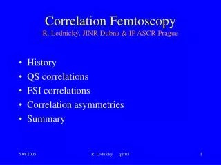
Correlation Femtoscopy R. Lednický, JINR Dubna & IP ASCR Prague. History QS correlations FSI correlations Correlation asymmetries Summary. History. Correlation femtoscopy :. measurement of space-time characteristics R, cï´ ~ fm. of particle production using particle correlations.

E N D
Correlation Femtoscopy R. Lednický, JINR Dubna & IP ASCR Prague • History • QS correlations • FSI correlations • Correlation asymmetries • Summary R. Lednický qm'05
History Correlation femtoscopy : measurement of space-time characteristics R, c ~ fm of particle production using particle correlations GGLP’60: observed enhanced ++, vs + at small opening angles – interpreted as BE enhancement KP’71-75: settled basics of correlation femtoscopy in > 20 papers • proposed CF= Ncorr /Nuncorr& mixing techniques to construct Nuncorr • clarified role of space-time characteristics in various production models • noted an analogy Grishin,KP’71 & differences KP’75 with HBT effect in Astronomy (see also Shuryak’73, Cocconi’74)
QS symmetrization of production amplitude total pair spin p1 2 CF=1+(-1)Scos qx x1 ,nns,s x2 1/R0 1 p2 2R0 nnt,t q =p1- p2 , x = x1- x2 |q| 0
Intensity interferometry of classical electromagnetic fields in AstronomyHBT‘56 product of single-detector currentscf conceptual quanta measurement two-photon counts p1 Correlation ~ cos px34 x1 x3 p-1 p2 x4 x2 detectors-antennas tuned to mean frequency star | x34 | Space-time correlation measurement in Astronomy source momentum picture p= star angular radius no info on star lifetime orthogonalto KP’75 momentum correlation measurement in particle physics source space-time picture x
momentum correlation (GGLP,KP) measurements are impossible in Astronomy due to extremely large stellar space-time dimensions while • space-time correlation (HBT) measurements can be realized also in Laboratory: Intensity-correlation spectroscopy Goldberger,Lewis,Watson’63-66 Measuring phase of x-ray scattering amplitude Fetter’65 & spectral line shape and width Glauber’65 Phillips, Kleiman, Davis’67: linewidth measurement from a mercurury discharge lamp 900 MHz t nsec
GGLP’60 data plotted as CF p p 2+ 2 - n0 R0~1 fm
3-dim fit: CF=1+exp(-Rx2qx2 –Ry2qy2-Rz2qz2-Rxzqxqz) Examples of present data: NA49 & STAR Correlation strength or chaoticity Interferometry or correlation radii STAR KK NA49 Coulomb corrected z x y
“General” parameterization at |q| 0 Particles on mass shell & azimuthal symmetry 5 variables: q = {qx , qy , qz} {qout , qside , qlong}, pair velocity v = {vx,0,vz} q0 = qp/p0 qv = qxvx+ qzvz y side Grassberger’77 RL’78 x out transverse pair velocity vt z long beam cos qx=1-½ (qx)2…exp(-Rx2qx2 –Ry2qy2-Rz2qz2-Rxz2qx qz) Interferometry radii: Rx2 =½ (x-vxt)2 , Ry2 =½ (y)2 , Rz2 =½ (z-vzt)2 Podgoretsky’83;often called cartesian or BP’95 parameterization
f (degree) KP (71-75) … Probing source shape and emission duration Static Gaussian model with space and time dispersions R2, R||2, 2 Rx2 = R2 +v22 Ry2 = R2 Rz2 = R||2 +v||22 Emission duration 2 = (Rx2- Ry2)/v2 If elliptic shape also in transverse plane RyRsideoscillates with pair azimuth f Rside2 fm2 Out-of plane Circular In-plane Rside(f=90°) small Out-of reaction plane A Rside (f=0°) large In reaction plane z B
Probing source dynamics - expansion Dispersion of emitter velocities & limited emission momenta (T) x-p correlation: interference dominated by pions from nearby emitters Resonances GKP’71 .. Interference probes only a part of the source Strings Bowler’85 .. Interferometry radii decrease with pair velocity Hydro Pratt’84,86 Kolehmainen, Gyulassy’86 Makhlin-Sinyukov’87 Pt=160MeV/c Pt=380 MeV/c Bertch,Gong, Tohyama’88 Hama, Padula’88 Pratt, Csörgö, Zimanyi’90 Rout Rside Mayer, Schnedermann, Heinz’92 Rout Rside ….. Collective transverse flow t RsideR/(1+mtt2/T)½ Longitudinal boost invariant expansion during proper freeze-out (evolution) time 1 in LCMS } Rlong(T/mt)½/coshy
AGSSPSRHIC: radii Clear centrality dependence Weak energy dependence STAR Au+Au at 200 AGeV 0-5% central Pb+Pb or Au+Au
AGSSPSRHIC: radii vs pt Central Au+Au or Pb+Pb Rlong:increases smoothly & points to short evolution time ~ 8-10 fm/c Rside,Rout: change little & point to strong transverse flow t~ 0.4-0.6 & short emission duration ~ 2 fm/c
Interferometry wrt reaction plane STAR’04 Au+Au 200 GeV 20-30% Typical hydro evolution p+p+ & p-p- Out-of-plane Circular In-plane Time STAR data: oscillations like for a static out-of-plane source stronger then Hydro & RQMD Short evolution time
Expected evolution of HI collision vs RHIC data Bass’02 QGP and hydrodynamic expansion hadronic phase and freeze-out initial state pre-equilibrium hadronization Kinetic freeze out dN/dt Chemical freeze out RHIC side & out radii: 2 fm/c Rlong & radii vs reaction plane: 10 fm/c 1 fm/c 5 fm/c 10 fm/c 50 fm/c time
Hydro assuming ideal fluid explains strong collective () flows at RHIC but not the interferometryresults Puzzle ? But comparing Bass, Dumitru, .. 1+1D Hydro+UrQMD 1+1D H+UrQMD Huovinen, Kolb, .. 2+1D Hydro with 2+1D Hydro Hirano, Nara, .. 3D Hydro kinetic evolution ? not enough t ~ conserves Rout,Rlong & increases Rside at small pt (resonances ?) Good prospect for Hirano .. 3DH + hadron transport + ? initial t
Why ~ conservation of spectra & radii? Sinyukov, Akkelin, Hama’02 Based on the fact that the known analytical solution of nonrelativistic BE with spherically symmetric initial conditions coincides with free streaming ti’= ti +T, xi’= xi+ vi T , vi v =(p1+p2)/(E1+E2) they proposed that the kinetic evolution can be close to free streaming alsoin realconditionsand thus ~ conserve the spectra and lead to small ~ conserved interferometry radii qxi’ qxi +q(p1+p2)T/(E1+E2) = qxi ~ justifies hydro motivated freezeout parametrizations
Checks with kinetic model Amelin, RL, Malinina, Pocheptsov, Sinyukov’05: System cools & expands but initial Boltzmann momentum distribution & interferomety radii are conserved due to developed collective flow
Hydro motivated parametrizations BlastWave: Schnedermann, Sollfrank, Heinz’93 Retiere, Lisa’04 Kniege’05
Au-Au 200 GeV Retiere@LBL’05 T=106 ± 1 MeV <bInPlane> = 0.571 ± 0.004 c <bOutOfPlane> = 0.540 ± 0.004 c RInPlane = 11.1 ± 0.2 fm ROutOfPlane = 12.1 ± 0.2 fm Life time (t) = 8.4 ± 0.2 fm/c Emission duration = 1.9 ± 0.2 fm/c c2/dof = 120 / 86
Buda-Lund: Csanad, Csörgö, Lörstad’04 Other parametrizations Similar to BW but T(x) & (x) hot core ~200 MeV surrounded by cool ~100 MeV shell Describes all data: spectra, radii, v2() Krakow: Broniowski, Florkowski’01 Single freezeout model + Hubble-like flow + resonances Describes spectra, radii but Rlong ? may account for initial t Kiev-Nantes: Borysova, Sinyukov, volume emission Erazmus, Karpenko’05 Generalizes BW using hydro motivated closed freezeout hypersurface Additional surface emission introduces x-t correlation helps to desribe Rout surface emission at smaller flow velocity Fit points to initial t of ~ 0.3
|-k(r)|2 Similar to Coulomb distortion of -decay Fermi’34: RL, Lyuboshitz’82 eq. time condition |t*| r*2 Final State Interaction fcAc(G0+iF0) s-wave strong FSI FSI } nn e-ikr -k(r) [ e-ikr +f(k)eikr/r ] CF pp Coulomb |1+f/r|2 kr+kr F=1+ _______ + … eicAc ka } } Bohr radius Coulomb only Point-like Coulomb factor k=|q|/2 FSI is sensitive to source size r and scattering amplitude f It complicates CF analysis but makes possible Femtoscopy with nonidentical particlesK,p, .. & Coalescence deuterons, .. Study “exotic” scattering,K, KK,, p,, .. Study relative space-time asymmetriesdelays, flow
Lyuboshitz-Podgoretsky’79: KsKs from KK also show FSI effect on CF of neutral kaons Goal: no Coulomb. But R may go up by ~1 fm if neglected FSI in BE enhancement KK (~50% KsKs) f0(980) & a0(980) STAR data on CF(KsKs) RL-Lyuboshitz’82 couplings from Martin’77 Achasov’01,03 no FSI l = 1.09 0.22 R = 4.66 0.46 fm 5.86 0.67 fm t
Long tails in RQMD: r* = 21 fm for r* < 50 fm NA49 central Pb+Pb 158 AGeV vs RQMD 29 fm for r* < 500 fm Fit CF=Norm[Purity RQMD(r* Scaler*)+1-Purity] RQMD overestimatesr* by 10-20% at SPS cf ~ OK at AGS worse at RHIC Scale=0.76 Scale=0.92 Scale=0.83 p
Goal: No Coulomb suppression as in pp CF & p CFs at AGS & SPS & STAR Wang-Pratt’99 Stronger sensitivity to R singlet triplet Scattering lengths, fm: 2.31 1.78 Fit using RL-Lyuboshitz’82 with Effective radii, fm: 3.04 3.22 consistent with estimated impurity R~ 3-4 fm consistent with the radius from pp CF STAR AGS SPS =0.50.2 R=4.50.7 fm R=3.10.30.2 fm
Correlation study of particle interaction +& & pscattering lengthsf0 from NA49 and STAR Fits using RL-Lyuboshitz’82 pp STAR CF(p) data prefer Ref0(p)< Ref0(pp) 0 NA49 CF(+) vs RQMD with SI scale:f0siscaf0 (=0.232fm) - sisca = 0.60.1 compare ~0.8 from SPT & BNL data E765 K e NA49 CF() data prefer |f0()| f0(NN) ~ 20 fm
Correlation asymmetries CF of identical particles sensitive to terms evenin k*r* (e.g. through cos 2k*r*) measures only dispersion of the components of relative separation r* = r1*- r2*in pair cms • CF of nonidentical particles sensitive also to terms odd in k*r* • measures also relative space-time asymmetries - shifts r* RL, Lyuboshitz, Erazmus, Nouais PLB 373 (1996) 30 Construct CF+x and CF-x with positive and negativek*-projectionk*x on a given directionx and study CF-ratio CF+x/CFx
Simplified idea of CF asymmetry(valid for Coulomb FSI) Assume emitted later than p or closer to the center x v Longer tint Stronger CF v1 CF k*x > 0 v > vp p p v2 k*/= v1-v2 x Shorter tint Weaker CF v CF v1 k*x < 0 v < vp p v2 p
CF-asymmetry for charged particles Asymmetry arises mainly from Coulomb FSI CF Ac() |F(-i,1,i)|2 =(k*a)-1, =k*r*+k*r* r*|a| F 1+ = 1+r*/a+k*r*/(k*a) k*1/r* } ±226 fm for ±p ±388 fm for +± Bohr radius k* 0 CF+x/CFx 1+2 x* /a x* = x1*-x2* rx* Projection of the relative separation r* in pair cms on the direction x x* = t(x - vtt) In LCMS (vz=0) or x || v: CF asymmetry is determined by space and time asymmetries
Usually: x and t comparable RQMD Pb+Pb p +X central 158 AGeV : x = -5.2 fm t = 2.9 fm/c +p-asymmetry effect 2x*/a -8% x* = -8.5 fm Shift x in out direction is due to collective transverse flow & higher thermal velocity of lighter particles xp > xK > x > 0 x RL’99-01 out tT F tT = flow velocity = transverse thermal velocity side t t = F+tT = observed transverse velocity y F xrx= rtcos =rt (t2+F2-tT2)/(2tF) mass dependence yry= rtsin = 0 rt zrz sinh = 0 in LCMS & Bjorken long. exp. measures edge effectat yCMS 0
pion BW Retiere@LBL’05 Distribution of emission points at a given equal velocity: - Left, bx = 0.73c, by = 0 - Right, bx = 0.91c, by = 0 Dash lines: average emission Rx Rx(p) < Rx(K) < Rx(p) px = 0.3 GeV/c px = 0.15 GeV/c Kaon px = 0.53 GeV/c px = 1.07 GeV/c For a Gaussian density profile with a radius RG and flow velocity profile F(r) = 0r/ RG RL’04, Akkelin-Sinyukov’96: x = RG bx0/[02+T/mt] Proton px = 1.01 GeV/c px = 2.02 GeV/c
NA49 & STAR out-asymmetries Au+Au central sNN=130 GeV Pb+Pb central 158 AGeV not corrected for ~ 25% impurity corrected for impurity r* RQMD scaled by 0.8 p K p Mirror symmetry (~ same mechanism for and mesons) RQMD, BW ~ OK points to strong transverse flow (t yields ~ ¼ of CF asymmetry)
Summary • Wealth of data on correlations of various particle species (,K0,p,,) is available & gives unique space-time info on production characteristics including collective flows • Rather direct evidence for strong transverse flow in HIC at SPS & RHIC comes from nonidentical particle correlations • Weak energy dependence of correlation radii contradicts to 2+1D hydro& transport calculations which strongly overestimate out&long radii at RHIC. However, a good perspective seems to be for 3D hydro& transport ? • A number of succesful hydro motivated parametrizations give useful hints for the microscopic models • Info on two-particle strong interaction: & & pscattering lengths from HIC at SPS and RHIC. Good perspective at RHIC and LHC
Apologize for skipping • Coalescence data (new d, d from NA49) • Problem of non-Gaussian form Csörgö .. • Imaging technique Brown, Danielewicz, .. • Correlations of penetrating probes • Comparison of different colliding systems • Multiple FSI effects Wong, Zhang, ..; Kapusta, Li; Cramer, .. • Spin correlations Alexander, Lipkin; RL, Lyuboshitz • ……
collective flow chaotic source motion x2-p correlation yes yes Teff with m yes yes R with mt yes yes x-p correlation yes no x 0 yes no CF asymmetry yes yes if t 0