Multilevel modeling in R

1. Multilevel modeling in R Tom Dunn and Thom Baguley, Psychology, Nottingham Trent University Thomas.Baguley@ntu.ac.uk

2. 1. Models for repeated measures or clustered data

3. Repeated measures ANOVA Usual practice is psychology is to analyze repeated measures data using ANOVA: One-way independent measures One-way repeated measures

4. Limitations of standard approaches e.g., repeated measures ANOVA • sphericity or multi-sample sphericity assumptions • dealing with non-orthogonal predictors e.g., time-varying covariates in RM ANOVA • dealing with missing values • treating items as fixed effects (e.g., Clark, 1973) • the problem of categorization • the problem of aggregation/disaggregation

5. Avoid repeated measures regression! Repeated measures regression is one attempt to deal with limitations of ANOVA such as non-orthogonal predictors e.g., using manual dummy coding (Lorch & Myers, 1990; Pedhazur, 1982) • data hungry (each indicator requires 1 df) • assumes sphericity; fixed effects • less flexible, powerful than multilevel models (Misangyi et al., 2006)

6. Multilevel models with random intercepts A random intercept model has predictors with fixed effects only: e.g., fixed random … or combined in single equation:

8. Random effects in multilevel models In the random intercept model the individual differences at level 2 are (like the random error at level 1) assumed to have a normal distribution: Individual differences in the effect of a predictor can also be modeled this way:

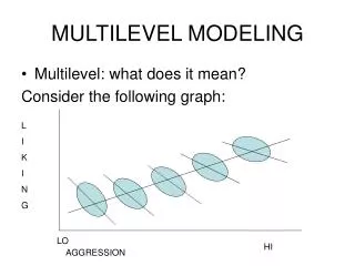
10. Example - voice pitch (1) How is male voice pitch is related to subjective attractiveness of a female face?† - 30 male participants - 32 female faces - ratings of attractiveness (1-9) in 2 contexts - potential time-varying covariates (e.g., baseline measure) Classical ANOVA: i) treats participants (but not faces) as random sample • can't incorporate time-varying covariates • aggregates data (effective n = 30 per context) † Data from Dunn, Wells and Baguley (in prep) and in Baguley (2012)

11. Example - voice pitch (1) contd. library(nlme) pitch.ri <- lme(pitch ~ base + attract, random=~ 1|Participant, data=pitch) summary(pitch.ri) Linear mixed-effects model fit by REML Data: pitch Log-restricted-likelihood: -7061.513 Fixed: pitch ~ base + attract (Intercept) base attract 89.5863997 0.2091518 0.4654556 Random effects: Formula: ~1 | Participant (Intercept) Residual StdDev: 13.05003 9.214851 Number of Observations: 1920 Number of Groups: 30

12. Modeling covariance matrices 1 In a two level random-intercept model the covariance structure is: This, in effect, assumes a form of compound symmetry of the repeated measures (with equal variances and covariances all zero)

13. Modeling covariance matrices 2 In a two level random-slope model with one predictor random at level 2 the covariance matrix is: In a repeated measures design this models the individual differences in the effect of the predictor (as well as its covariance with the intercept).

14. Unstructured covariance matrices In repeated measures it is possibly to have an unconstrained covariance matrix at the participant level (usually level 2). This is an example for four measurement occasions: In this kind of unstructured matrix there are no assumptions about the form of the matrix (e.g., sphericity, compound symmetry or multisample sphericity)

15. Example - random effect of voice pitch (2) Attractiveness might not have a fixed effect (in fact it is more likely that it varies between people) lme(pitch ~ base + attract, random=~ attract|Participant, data=pitch) AIC BIC logLik 14133.03 14160.82 -7061.513 Random effects: Formula: ~1 | Participant (Intercept) Residual StdDev: 13.05003 9.214851 Fixed effects: pitch ~ base + attract Value Std.Error DF t-value p-value (Intercept) 89.58640 5.537340 1888 16.178598 0 base 0.20915 0.044474 1888 4.702804 0 attract 0.46546 0.104619 1888 4.449042 0

18. 2. Estimation and inference

19. Estimation in multilevel models Estimation is iterative and usually uses maximum likelihood (as with logistic regression): - IGLS or FML (iterative generalized least squares) - RIGLS or RML (restricted maximum likelihood estimation) - Parametric bootstrapping - Non-parametric bootstrapping - MCMC (Markov chain Monte Carlo methods)

20. Comparing models Confidence intervals and tests - deviance (likelihood ratio) tests (-2LL or change in -2 log likelihood has approximate χ2 distribution) • Wald tests and CIs (estimate/SE has approximate z distribution) Information criteria • AIC, BIC or (MCMC derived) DIC (-2LL with a penalty for number of parameters)

21. Accurate inference … - for standard repeated measures ANOVA models it is possible to use t and Fstatistics • if a complex covariance structure (anything other than compound symmetry) or unbalanced model is used then inference is problematic owing to: a) difficulty estimating the error df b) boundary effects (for variances)

22. Possible solutions - asymptotic approximations (in large samples)* • corrections such as the Kenwood-Rogers approximation (e.g., using pbkrtest) • bootstrapping* • MCMC estimation (e.g., using lme4 or MCMCglmm)* * e.g., see Baguley (2012) for examples

23. Requirements for accurate estimation Centering predictors • essential to use appropriate centering strategy in random slope models see Enders & Tofighi (2007) Nested versus fully-crossed structures • many experimental designs in psychology are fully crossed see Baayen et al. (2008) Estimation, sample size and bias • sample size at highest level of model is crucial see Hox (2002), Maas & Hox (2005)

24. Nested versus fully crossed structures In nested structures lower level units occur in only one higher level unit e.g., children in schools In fully crossed structures ‘lower’ level units are observed within all ‘higher’ level units e.g., same 32 faces used for all 30 participants Baayen et al. (2006) argue that many researchers incorrectly model fully crossed structures as nested

26. Example - fully crossed model (3) detach(package:nlme) ; library(lme4) lmer(pitch ~ base + attract + (1|Participant) + (1|Face), data=pitch) † Formula: pitch ~ base + attract + (1 | Participant) + (1 | Face) AIC BIC logLik deviance REMLdev 14134 14167 -7061 14118 14122 Random effects: Groups Name Variance Std.Dev. Face (Intercept) 0.44417 0.66646 Participant (Intercept) 171.72946 13.10456 Residual 84.47292 9.19092 Number of obs: 1920, groups: Face, 32; Participant, 30 Fixed effects: Estimate Std. Error t value (Intercept) 90.03032 5.54083 16.249 base 0.20543 0.04447 4.620 attract 0.45910 0.11229 4.088 lmer(pitch ~ base + attract + (attract|Participant) + (1|Face), data=pitch) † Assumes that the fully crossed structure is correctly coded in the data set

27. Advantages of multilevel approaches • often greater statistical power (e.g., for RM ANOVA) • multiple random factors (nested or crossed) • copes with non-orthogonal predictors • copes with time-varying covariates • assumes missing outcomes are MAR (not MCAR) • explicitly models variances and covariances