ESTIMATION
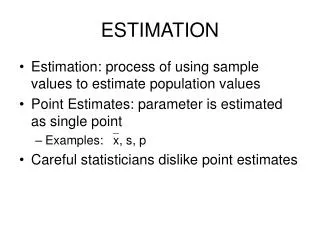
ESTIMATION. Estimation: process of using sample values to estimate population values Point Estimates: parameter is estimated as single point Examples: x, s, p Careful statisticians dislike point estimates. Interval Estimates.

ESTIMATION
E N D
Presentation Transcript
ESTIMATION • Estimation: process of using sample values to estimate population values • Point Estimates: parameter is estimated as single point • Examples: x, s, p • Careful statisticians dislike point estimates
Interval Estimates • Example: there is a 90% probability that somewhere between 58 and 68% of Americans oppose same-sex marriage • Draws explicit attention to the fact of variability in the sample results; avoids putting too much weight on one number
Think about the interval 42 – 1.64 * 1 to 42 + 1.64 * 1: This interval contains 90% of the sample means that could ever be drawn from this population
The interval 40.36 to 43.64 contains 90% of the sample means possible from this population • No sample mean in this interval differs from μ by more than 1.64 grams • Hence, there is a 90% probability that any arbitrary x differs from μ by no more than 1.64 • Thus, there is a 90% probability that μ is in the interval x 1.64
Look at this interval • x 1.64 * 1 • 1.64 is a z value, chosen to correspond to 90%, the confidence level • 1 is the standard error of the mean • So the width of the interval is set by the confidence level (which determines number of standard errors in interval) and the standard error, the measure of variation in sample means
A C% Confidence Interval for the Population Mean When σ Is Known
Examples: • A population of Christmas trees has unknown mean with σ = 4. For a sample of 25 trees, the sample mean = 16.6 ft. Calculate a 95% confidence interval for the population mean.
Same data: calculate a 90% confidence interval • Same data: suppose that we increase sample size to 81
Width of Confidence Interval Depends On • Confidence level: as C increases, width decreases • Sample size: as n increases, width decreases • Variability in population: as σ increases, standard error increases and width of interval increases
The quantity zC * σX is called the maximum error in the estimate • The quantity 2 * zC * σX is called the precision in the estimate • this quantity is the width of the confidence interval
FINDING THE RIGHT SAMPLE SIZE • Sometimes we wish to hold the error in the estimate within some limit • Define e = zC * σX or substituting Solve this expression for n, yielding
Example: With σ = 4 and 95% confidence level, we require that the maximum error in the estimate be no more than 0.5 ft. What sample size is necessary?
Examples: • Expectations of inflation are known to be normally distributed with standard deviation = 1.2%. A survey of sixty households found a sample average expectation of 4% inflation for the coming year. Calculate a 98% confidence interval for the population’s expectation of inflation in the coming year.
If we require a maximum error in the estimate of 0.1%, how large a sample must we take? • Cigarette filters have a “process” standard deviation of 0.3 mm with normal distribution. The current mean is unknown, but a sample of 25 filters have a mean of 20 mm. • Calculate a 90% confidence interval for the population mean • Find the sample size necessary to hold the error in the estimate to 0.04 mm
Student’s t distribution • Suppose σ is NOT known; then we are not entitled to use a z value in calculating confidence intervals • If, however • The population is known to be normally distributed OR • The sample size is large enough to invoke the Central Limit Theorem, then we use • A value drawn from the t distribution
Hey, Prof, what’s a t distribution? • Characteristics • Symmetric about its mean of zero • Values tend to cluster in the center, producing a bell shaped curve • Differences from z: • Fatter tails and less mass in the center • There is a family of t distributions, based on “degrees of freedom”
Degrees of freedom: the sample size minus number of parameters to be estimated before estimating a variance Before estimating the variance, we must first calculate x-bar, an estimate of the population mean: we lose one degree of freedom, leaving us with n – 1 degrees of freedom
Confidence Intervals with the t distribution: Where t is chosen for the desired confidence level and has n – 1 degrees of freedom
Examples: • Seven male students are allowed to imbibe their favorite beverage until they are visibly inebriated. The amounts consumed in ounces are: 3.7, 2.9, 3.2, 4.1, 4.6, 2.3, 2.5. Calculate a 95% confidence interval for the amount of the drink it would take to get the average member of the population drunk.
Calculate x-bar and s • Then calculate the sample standard error • Find t for 6 degrees of freedom and = 0.025 • Finally, calculate the confidence interval
In a sample of 41 students who work, the sample mean is 16.561 hours and s = 5.7128 hours. The distribution appears to be somewhat skewed upwards. Find a 90% confidence interval for the average hours worked by all ASU students who work.
USE OF THE t DISTRIBUTION • Footnote: Who was “Student”? A pseudonym for William Gosset • The t is often thought of as a small-sample technique • But, STRICTLY SPEAKING, the t should be used whenever the population standard deviation σ is NOT KNOWN • Some practitioners use z whenever the sample is large • Central Limit Theorem • There isn’t much difference between t and z
Notes: • For large samples with σ unknown, different practitioners may proceed differently. Some argue for using a z, appealing to CLT. Others use a t since it gives a less precise estimate. For this course: use a t whenever the population standard deviation is not known. • Small samples from non-normal populations are beyond the scope of this course
Confidence intervals for the population proportion • Sample proportion p = x/n • E(p) = and In general is not know, so must be estimated with p and we use
Then the confidence interval is • p zC sp • Note that proportion problems always use a z value • Normal approximates binomial • EXAMPLE: Of 112 students in a sample, 70 have paying jobs. Calculate a 95% confidence interval for the proportion in the population with paying jobs.
p = 70/112 = 0.625 • 0.625 1.96 * 0.045 etc. • 0.625 0.089660819 or 0.625 0.09 • We are 95% confident that 0.54 0.71
EXAMPLE: • In a sample of 320 professional economists, 251 agreed that “offshoring” jobs is good for the American economy. Calculate a 90% confidence interval for the proportion in the population of professional economists who hold this view.
Finding the Right Sample Size • The error in the estimate is given by zC σp or, substituting Solving for n yields:
In general is not known • Two solutions: • Assume = 0.5 • Result is the largest sample that would ever be needed • Conduct a pilot study and use the resulting p as an estimate of • May give a somewhat smaller sample size if p is much different from 0.5 • Saves sampling cost
Example: • Above we had a 95% confidence interval with n = 112 of 0.625 0.09 or a 9% error. Suppose we require a maximum error of 3%. • Approach 1: let = 0.5
Approach 2: assume = 0.625 The difference is more dramatic if p is much different from 0.5. In a random sample of 300 students in NC, 30 have experienced “study” abroad. A 95% confidence interval for the population proportion is 10% 3.4%. Suppose we require a maximum error of 2%. Approach 1 gives _______ and approach 2 gives _________.