Estimation

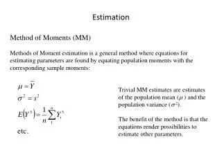
1. Estimation Method of Moments (MM) Methods of Moment estimation is a general method where equations for estimating parameters are found by equating population moments with the corresponding sample moments: Trivial MM estimates are estimates of the population mean ( ) and the population variance ( 2). The benefit of the method is that the equations render possibilities to estimate other parameters.

2. Mixed moments • Moments can be raw (e.g. the mean) or central (e.g. the variance). • There are also mixed moments like the covariance and the correlation (which are also central). • MM-estimation of parameters in ARMA-models is made by equating the autocorrelation function with the sample autocorrelation function for a sufficient number of lags. • For AR-models: Replace kby rk in the Yule-Walker equations • For MA-models: Use developed relationships between k and the parameters • 1 , … , qand replace kby rk in these. • Leads quickly to complicated equations with no unique solution. • Mixed ARMA: As complicated as the MA-case

3. Example of formulas AR(1): AR(2):

4. MA(1): Only one solution at a time gives an invertible MA-process

5. The parameter e2: Set 0 = s2 

6. Example Simulated from the model >ar(yar1,method="yw") Call: ar(x = yar1, method = "yw") Coefficients: 1 0.2439 Order selected 1 sigma^2 estimated as 4.185 “Yule-Walker (leads to MM-estimates)

7. Least-squares estimation Ordinary least-squares Find the parameter values p1, … , pm that minimise the square sum where X stands for an array of auxiliary variables that are used as predictors for Y. Autoregressive models The counterpart of S (p1, … , pm ) is Here, we take into account the possibility of a mean different from zero.

8. Now, the estimation can be made in two steps: • Estimate  by • Find the values of 1 , …, p that minimises The estimation of the slope parameters thus becomes conditional on the estimation of the mean. The square sum Sc is therefore referred to as the conditional sum-of-squares function. The resulting estimates become very close to the MM-estimate for moderately long series.

9. Moving average models More tricky, since each observed value is assumed to depend on unobservable white-noise terms (and a mean): As for the AR-case, first estimate the mean and then estimate the slope parameters conditionally on the estimated mean, i.e. For an invertible MA-process we may write

10. The square sum to be minimized is then generally • Problems: • The representation is infinite, but we only have a finite number of observed values • Sc is a nonlinear function of the parameters 1 , … , q Numerical solution is needed Compute et recursively using the observed values Y1, … , Yn and setting e0 = e–1 = … = e–q = 0 : for a certain set of values 1 , … , q Numerical algorithms used to find the set that minimizes

11. Mixed Autoregressive and Moving average models Least-squares estimation is applied analogously to pure MA-models. et –values are recursively calculated setting ep= ep – 1 = … = ep + 1 – q = 0 Least-squares generally works well for long series For moderately long series the initializing with e-values set to zero may have too much influence on the estimates.

12. Maximum-Likelihood-estimation (MLE) For a set of observations y1, … , yn the likelihood function (of the parameters) is a function proportional to the joint density (or probability mass) function of the corresponding random variables Y1, … , Yn evaluated at those observations: For a times series such a function is not the product of the marginal densities/probability mass functions. We must assume a probability distribution for the random variables. For time series it is common to assume that the white noise is normally distributed, i.e.

13. with known joint density function For the AR(1) case we can use that the model defines a linear transformation to form Y2, …, Yn from Y1, …, Yn–1 and e2, …, en This transformation has Jacobian = 1 which simplifies the derivation of the joint density for Y2, …, Yngiven Y1to

14. Now Y1 should be normally distributed with mean  and variance e2/(1–2) according to the derived properties and the assumption of normally distributed e. Hence the likelihood function becomes and the MLEs of the parameters  .  and e2 are found as the values that maximises L

15. Compromise between MLE and Conditional least-squares: Unconditional least-squares estimates of  and  are found by minimising The likelihood function can be put up for ant ARMA-model, however it is more involved for models more complex than AR(1). The estimation need (with a few exceptions) to be carried out numerically

16. Properties of the estimates Maximum-Likelihood estimators has a well-established asymptotic theory: Hence, by deriving large-sample expressions for the variances of the point estimates, these can be used to make inference about the parameters (tests and confidence intervals) See the textbook

17. Model diagnostics • Upon estimation of a model, its residuals should be checked as usual. • Residuals should be plotted in order to check for • constant variance (plot them against predicted values) • normality (Q-Q-plots) • substantial residual autocorrelation (SAC and SPAC plots)

18. Ljung-Box test statistic Let and define If the correct ARMA(p,q)-model is estimated, then Q*,Kfollows a Chi-square distribution with K – p– q degrees of freedom. Hence, excessive values of this statistic indicates that the model has been erroneously specified. The value of K should be chosen large enough to cover what can be expected to be a set of autocorrelations that are unusually high if the model is wrong.