Download
1 / 25
250 likes | 415 Views
Variability of the Australian Wave Climate. Mark Hemer Informal Oceanography Seminar 14-Sep-2006 CSIRO Marine and Atmospheric Research. Coastal erosion and climate change. Warming Oceans and Climate. Changes to weather systems and storms. Sea-level rise. CHANGING RISK OF COASTAL EROSION

E N D
Variability of the Australian Wave Climate Mark Hemer Informal Oceanography Seminar 14-Sep-2006 CSIRO Marine and Atmospheric Research
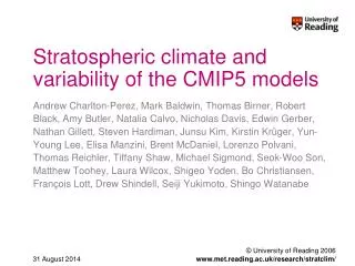
Coastal erosion and climate change Warming Oceans and Climate Changes to weather systems and storms Sea-level rise CHANGING RISK OF COASTAL EROSION (Felt most acutely via extreme events – storm surges and large wave events) Wamberal, NSW, 1978 Fairy Bower, Manly 2003 Gold Coast, 1967
Beach-face junction swash wave setup R Ej E Measured Tide Level ET Datum Potential Impacts of a changing wave climate Coastal Erosion – impacting coastal infrastructure and supra-tidal habitats: Wave-induced erosion of sea-cliffs or sand dunes occurs if E = (ET + R) > Ej Recent position paper (Woodworth et al., 2006) indicates waves are an important consideration, as wave setup alone can be of order 0.5m
Other wave climate studies • Global studies • Young and Gorman (1996) Atlas of the Oceans: Wind and Wave Climate • Caires and Sterl (2005) The web-based KNMI/ERA-40 Wave Atlas • Cox and Swail (2001) A global wave hindcast over the period 1958-1997. • Gulev (2004) Trends in wave climate observed from voluntary observing ships • Regional Studies • Woolf et al. (2001) variability and predictability of waves in the North Atlantic • Gormal et al., (2002) New Zealand Wave hindcast model • Laing et al. (1998) New Zealand wave climate from satellite observations • Sasaki et al (2005) recent changes in summertime extreme wave heights in the Western North Pacific. • Australian Studies • Short, A. (2000) Narabeen Beach Rotation correlation to El-Nino • Castelle (2006) Wave-climate changes at the Gold Coast • Callaghan (2006) Coastal erosion and inundation due to severe storm changes in NSW. • Tomlinson (2005) Coastal Erosion on East Coast of Australia • GA (2005) Perth Coastal Erosion study • Goodwin (2005) mean wave direction climatology for southeastern Australia • JCU (2004) GBR Wave Atlas
Objectives • To determine a climatology of the offshore wave conditions in the Australian region by combining satellite altimeter data, global wave model data, and Australian wave-rider buoys. • To identify variability and trends in the offshore wave climate, and in the intensity and frequency of extreme wave events in the Australian region (and determine the drivers of this variability). • Estimate the coastal response to these historical changes in wave-climate using regional wave models for selected regions. Where wave climate describes the height, length and direction of surface ocean waves
ERA-40 Global WAM Model 45 year hindcast Sep-1957 – Aug-2002 • Implementation of WAM wave model. Model run on 1.5° lat/lon grid • Variables of interest at 6-hourly intervals on 2.5°lat/lon gridfree of charge • Significant wave height • Mean Wave Period • Mean Wave Direction • 10 m u and v wind components • Mean sea level pressure • Data inhomogeneous in time. • 09/57 – 11/91, 06/93-12/93 No assimilated data • 12/91 – 05/93. faulty ERS-1 FDR assim • 01/94 – 05/96. good, un-callib ERS-1 FDR assim • 06-96 – ERS-2 FDR assim. • Caires & Sterl (2005). Non-parametric correction of ERA-40 wave data. Corrected (C-ERA-40) dataset. Caires et al. (2005) E40 wave atlas
NWW3 Global wave model 3rd generation spectral model (like WAM) (Tolman, 2002) • Global model 1.25d (lon) x 1.0d (lat) grid. (77dS – 77dN) • Forcing winds from GDAS and aviation cycle of MRF Model. • Includes bathymetry effects, variable ice, GDAS SST. • Variables archived since • 01/1997 at 3-hr int. • Significant wave height • Peak wave period • Mean wave direction Greater number of variables available operationally.
Australia’s existing waverider buoys Australian wave-rider buoy network 27 waverider buoys 10 directional 1st deployment: Pt. Kembla, NSW (1974) Latest addition: Esperance, WA (2006) Other available multi-year wave data
Satellite Altimeter measured wave variables • Data downloaded from TUD RADS database (and checked against local data) Time, lat, lon, SWH (Ku, C Band), so (Ku, C Band), std(SWH), std(so)
BoM visual sea-state records • Visual sea/swell state conditions reported several times daily. • Sea and swell state separated: Height (by code) and Direction. • 26 stns recording at present. 95 stns available with > 10 yr record. 6 stns with > 50 year record. • Cape Otway record commences in 1880. • 0 Calm-Glassy(0 m) • Calm-Rippled (0.1 m) • Smooth-Wavelet(0.1 - 0.5 m) • Slight (0.5 – 1.25 m) • Moderate(1.25 – 2.5 m) • Rough (2.5 – 4.0 m) • Very Rough(4.0 – 6.0 m) • High(6.0 – 9.0 m) • Very High(9.0 – 14.0 m) • Phenomenal(> 14.0 m) Photo: Lighthouses of Australia Inc
Summary of available wave data Data count (units) 1880 2006 Other data : NIWA hindcast wave model (pts), BoM archived wave model output.
Validity of ERA-40 Time window: 6 hours Nearest grid cell. Low RMSE at un-sheltered buoy locations Slope predominantly < 1 Y-Intercept predominantly positive Overestimates low wave heights, and Underestimates high wave heights (consistent with comparison to NDBC-NOAA buoys (Sterl & Caires, 2005) ALL DATA (N = 340494) RMSE = 0.782 m RPEARSONS = 0.744 Regression, HE = 0.722 HB + 0.8384 EXPOSED SITES ONLY (N = 390494) RMSE = 0.653 m RPEARSONS = 0.783 Regression, HE = 0.716 HB + 0.7697
Validity of C-ERA-40 Low RMSE at un-sheltered buoy locations ALL DATA (N = 368879) RMSE = 0.786 m RPEARSONS = 0.742 Regression, HCE = 0.864 HB + 0.587 EXPOSED SITES ONLY (N = 259843) RMSE = 0.601 m RPEARSONS = 0.810 Regression, HCE = 0.869 HB + 0.4505
Validity of NWW3 Low RMSE at un-sheltered buoy locations ALL DATA (N = 440489) RMSE = 0.910 m RPEARSONS = 0.793 Regression, HW = 0.901 HB + 0.711 EXPOSED SITES ONLY (N = 313762) RMSE = 0.692 m RPEARSONS = 0.870 Regression, HW = 0.955 HB + 0.4784
Validity of Altimeters All altimeter data within 30km radius of buoys. 6 hour time window. Corrections applied to altimeter according to existing correction formulae – derived from comps to NDBC-NOAA buoys (Challenor & Cotton, 2002) ALL DATA (N = 11962) RMSE = 0.738 m RPEARSONS = 0.818 Regression, HA = 0.904 HB + 0.434 EXPOSED SITES ONLY (N = 9874) RMSE = 0.714 m RPEARSONS = 0.815 Regression, HE = 0.922 HB + 0.3744
Validity of SS Problems: 1. Conversion from code to HS Method adopted (allowing best fit). H assigned for each Sea and swell code. If sea and swell recorded from same 30d sector, Hs = √(HSEA + HSWELL), else Hs = max(HSEA, HSWELL) 2. Low data count, as very few records with SS record near to buoy over same period. 3. Geographic differences between Coastal and offshore locations ALL DATA (N = 179240) RMSE = 1.604 m RPEARSONS = 0.535 Regression, HSS = 1.1127 HB + 0.626
5-yr wave climate (Hs) mean comparison ERA-40 C-ERA40 NWW3 Altimeters
5-yr Annual Cycle (regional means) ERA-40 C-ERA40 NWW3 Alt Alt: uncor
Patterns of variability (C-ERA40) • Applied an Empirical Orthogonal Function Analysis to 45yr record of: • Monthly anomaly data • (annual cycle removed) • 2. Annual mean data • 3. Annual summer mean data • 4. Annual autumn mean data • 5. Annual winter mean data • 6. Annual spring mean data • On 5 regions • Whole Aus region • NW • NE • SE • SW
Exploring drivers of inter-annual variability Exploring correlations between time-series of coefficients of EOFs and existing indices Correlation > 0.65 for: To SAMI PC3 (explaining 4.5% of variance) SW region, Annual summer mean. To SOI PC1 (explaining 61 % of variance) NE Region, Annual mean. No time lag currently considered. At present - SOI - SAMI To look at: - IOD, PDO(?) - wind anomalies Monthly mean Aus region (N=530) RSOI RSAMI -0.348 0.409 0.530 -0.376 0.109 -0.266 -0.197 -0.220 -0.067 -0.287 0.060 0.179
Previous studies of trends in HS(NSW and Qld Buoys) QEPA: Boswood et al. (2005) No significant trend in HS in Qld buoy data Lord & Kulmar (2000) 5-7mm/yr increase In NSW buoys Over 15 yr record
Trends in HSm (C-ERA40) Trend in Hsm in Australian region, in C-ERA40 record. 45 year record. (by season, and region) (m/yr) Annual DJF MAM JJA SON Aus 0.0044 0.0041 0.0061 0.0050 0.0025 NW 0.0022 0.0017 0.0032 0.0033 0.0008 NE 0.0027 0.0027 0.0046 0.0032 0.0003 SE 0.0053 0.0050 0.0074 0.0059 0.0029 SW 0.0074 0.0069 0.0094 0.0077 0.0055 • What does the altimeter record show for the region?
Trends in HS99 (C-ERA40) Trend in Hs99 in Australian region, in C-ERA40 record. 45 year record. (by season, and region) (m/yr) Annual DJF MAM JJA SON Aus 0.0080 0.0083 0.0116 0.0078 0.0041 NW 0.0041 0.0045 0.0063 0.0043 0.0012 NE 0.0078 0.0081 0.0115 0.0070 0.0044 SE 0.0095 0.0094 0.0109 0.0115 0.0064 SW 0.0112 0.0118 0.0176 0.0098 0.0054 • Can the altimeter record measure this, given the low sampling rate of altimeter wave measurements?
Partial conclusions & continuation • C-ERA40, WW3 and Altimeter are suitable datasets for describing Australian offshore wave climate • Speculatively (only observed in one dataset at present). • SOI correlated to wave heights in NE region. • SAMI correlated to wave heights in SW region. • Mean Sig, Wave heights in the AUS region increasing by 5-10mm/yr. • Max. Sig, Wave heights in the AUS region increasing twice as fast. • TO DO: • Repeat all of the above for H90, H99 • Repeat EOF & Trend Analyses using Altimeter dataset • Describe wave direction climate, and explore variability and trends. • Determine frequency of large wave events (exceedances). Explore variability and trends. • Coastal response to trends and variability.
If you would like to present one of these Thursday informal seminars - contact Thanks John Church, CSIRO NSW, Dept of Commerce. MHL John Hunter, ACECRC Port of Melbourne Australian Greenhouse Office NOAA Bureau of Meteorology ECMWF-ERA-40 QEPA Andreas Sterl, KNMI WA. DPI James Carley, WRL, UNSW Name: Mark HemerTitle: Climate processes post-docPhone: +61 3 6232 5017Email: mark.hemer@csiro.auWeb: www.cmar.csiro.au