Download
1 / 18
180 likes | 347 Views
Diagnostics Related to the Unwanted Beam. Pavel Evtushenko, Jlab FEL. Flavors of Unwanted beam. Four sorts of the unwanted beams Fraction of the phase space distribution that is far away from the core (due to the beam dynamics)

E N D
Diagnostics Related to the Unwanted Beam Pavel Evtushenko, Jlab FEL
Flavors of Unwanted beam Four sorts of the unwanted beams Fraction of the phase space distribution that is far away from the core (due to the beam dynamics) Low charge due to not well attenuated Cathode Laser (ERLs) – but real bunches that have proper timing for acceleration Due to the Cathode Laser but not properly timed (scattered and reflected light) Field emission: Gun (can be DC or RF), Accelerator itself (can be accelerated in both directions)
For the number 2-4 • First of all prevent as much as possible • Take care of the Cathode Laser going out of the gun • Use Brewster angle windows (polarization) or coatings (still 10-4) • Cathode that scatters less (optically flat) (requirement?) • Having load lock would help to keep cathode in optically good condition • Non UV cathodes (green) more favorable • Extinction ration of the EO cells: high and stable • Field emission … well … either it system is built well, or you run limited by FE (just so that you can tolerate it)
For the number 1 • Linacs with average current 1-2 mAand energy 1-2.5 GeVare envisioned as drivers for next generation high average brightness Light Sources (up to 5 MW beam power) vs. presently operational linac based X-ray sources 24 uA(FLASH) and 15 nA(LCLS) • JLab IR/UV Upgrade is a 9 mAERL with average beam power of 1.2 MW – provides us with operational experience of high current linac and is a good testing ground for future development • Halo - parts of the phase space with large amplitude and small intensity - is one of the limitations for high current linacs • Linac beams have neither the time nor the mechanism to come to equilibrium (unlike storage rings, which also run high current) • Besides Light Sources there is a number of linac application requiring high current operation with low or no beam halo
Measurements vs. Modeling at the level ~103 Measured in JLab FEL injector, local intensity difference of the core and “halo” is about 300. (500 would measure as well) 10-bit frame grabber & a CCD with 57 dB dynamic range PARMELA simulations of the same setup with 3E5 particles: X and Y phase spaces, beam profile and its projection show the halo around the core of about 3E-3. Even in idealized system (simulation) non-linear beam dynamics can lead to formation of halo.
Drive Laser “ghost” pulses • Using a Log-amp is an easy way to diagnose presence of the “ghost” pulses • Log-amps with dynamic range 100 dB are available 631 uA (100%) 135 pC x 4.678125 MHz 5.7 uA (~0.9 %) 37.425 MHz “ghost” pulses
Cathode Laser pulse via streak camera • appears to be close to Gaussian on linear scale; tails not so much Gaussian • the difference from Gaussian distribution is obvious on log scale • realistic (measured) distribution must be used for realistic modeling • especially is the calculations are intended for large dynamic range effects
“The Grand Scheme” I. Transverse beam profile measurements with LDR Wire scanner LDR imaging CW laser wire Coronagraph II. Transverse phase space measurementswith LDR III. Longitudinal phase space with LDR(in injector at 9 MeV) Drive Laser LDR measurements to start modeling with LDR and real Initial conditions • transverse • longitudinal • cathode Q.E. 2D Tomography – where linear optics work (135 MeV) Time resolving laser wire (Thomson scattering, CW) Scanning slit - space charge dominated beam (9 MeV) Transverse kicker cavity + spectrometer + LDR imaging IV. High order optics to manipulatehalo V. Beam dynamics modeling with LDR
Wire scanner measurements A. Freyberger, CEBAF measurements, in DIPAC05 proceedings • wire with diameter much smaller than the beam size interacts with beam as it is scanned across it • there is a number of interaction mechanisms: • beam capture • secondary emission • scattering • conversion • different ways to detect the signal • induced current • secondary particles (counting) • only 1D projections of 2D distributions • takes time (“patience limited”) • real LINAC beams – non-equilibrium
Wire scanner measurements A. Freyberger, CEBAF measurements, In DIPAC05 proceedings • wire with diameter much smaller than the beam size interacts with beam as it is scanned across it • there is a number of interaction mechanisms: • beam capture • secondary emission • scattering • conversion • different ways to detect the signal • induced current • secondary particles (counting) • only 1D projections of 2D distributions • takes time (“patience limited”) • real LINAC beams – non-equilibrium at JLab FEL
Large Dynamic Range imaging (1) • To explain the idea we consider JLab FEL tune-up beam and the use of OTR. • Beam – 250 μs macro pulses at 2 Hz, bunch rep. rate ~ 4.678 MHz, 135 pCbunch charge, ~ 158 nC integrated charge (limits the beam power to safe level) • With typical beam size of few hundred μm OTR signal is attenuated by ~ 10 to keep CCD from saturation. For phosphor or YAG:Ce viewers attenuation of at least 100 is used. Insertable ND1 and ND2 filters are used. • Quantitative OTR intensity measurements agrees well with calculations – well understood • With OTR there is enough intensity to measure 4 upper decades. Lower two decades need gain of about 100 to be measured. • The main principle is to use imaging with 2 or 3 sensors with different effective gain simultaneously and to combine data in one LDR image digitally • The key elements: • image intensifiers (necessary gain and higher is available) • accurate alignment and linearity • the algorithm, data overlap from different sensors • understanding CCD well overflow - transverse extend • Diffraction Effects in the optical system
Large Dynamic Range imaging (2) To be measured with imaging sensor #1 and attenuation ~ 10 Intensity range that can be measured now with no additional gain. To be measured with imaging sensor #2 and gain ~ 200 Intensity range where additional gain of ~ 100 is needed
Large Dynamic Range imaging (3) To be measured with imaging sensor #1 and attenuation ~ 10 Intensity range that can be measured now with no additional gain. To be measured with imaging sensor #2 and ~ no gain Intensity range where additional gain of ~ 100 is needed To be measured with imaging sensor #3 and gain ~ 200
CW laser wire (1) • wavelength conversion assuming: • beam energy 9 MeV • laser wavelength 1.55 μm differential cross section (angular extent dependence on the beam energies) initial wavelength 1.55 μm
CW laser wire (2) • wavelength conversion assuming: • beam energy 9 MeV • laser wavelength 1.55 μm differential cross section (angular extend dependent on the beam energies) wavelength range: 150 nm – 850 nm (to stay out of VUV And be able to use PMTs)
CW laser wire (3) • wavelength conversion assuming: • beam energy 9 MeV • laser wavelength 1.55 μm • photon rate • Assuming: • bunch charge 135 pC • laser wavelength 1.55 μm • pulse energy ~7 nJ • tlaser500 fs • tbeam2.5 ps • fbeam9.356 MHz • rlaser100 μm • We get Ns=0.02, but fs=174 kHz ! • There is factor of ~ 100 to be lost, • but there is also factor of ~100 to be • gained by pulse stacking. • Plus lock-in amplifier improves SNR as: wavelength range: 150 nm – 850 nm (to stay out of VUV And be able to use PMTs)
Conclusion / Outlook • The general approach of the program is the to: • develop and built diagnostics tools • study beam dynamics (phase space evolution) • implements beam optics for better manipulation of the halo • use the experimental data for modeling that is close to reality in sense of initial conditions (iterate between the experiments and the modeling)
JLab IR/UV ERL Light Source Ebeam135 MeV Bunch charge: 60 pC – UV FEL 135 pC – IR FEL Rep. rate up to 74.85 MHz 25 μJ/pulse in 250–700 nm UV-VIS 120 μJ/pulse in 1-10 μmIR