Download

1 / 56
560 likes | 707 Views
Use of Multi-Model Super-Ensembles in Hydrology. Martyn Clark * Steven Markstrom. Lauren Hay George Leavesley. Roland Viger U.S. Geological Survey Water Resources Discipline National Research Program * University of Colorado - Boulder. Hydrologic Simulation. Inputs Time series data

E N D
Use of Multi-Model Super-Ensembles in Hydrology Martyn Clark* Steven Markstrom Lauren Hay George Leavesley Roland Viger U.S. Geological Survey Water Resources Discipline National Research Program * University of Colorado - Boulder
Hydrologic Simulation • Inputs • Time series data • Precipitation, Minimum + Maximum Temperature • Parameters (static information) • Spatial characteristics • Non-spatial characteristics • Modeling Software
Sources of Error • State of the system: • observed != simulated • Error in: • Inputs • Time series data • Parameters • Modeling Software
Optimization of Model • Standard technique: • adjustment of parameters • Spatial characteristics • Non-spatial characteristics • “Fitting” simulated hydrograph to the observed hydrograph
Optimization of Model • Standard technique: • adjustment of parameters • Spatial characteristics • Non-spatial characteristics • “Fitting” simulated hydrograph to the observed hydrograph • Ignores numerous other sources of error!
Sources of Error • Inputs • Time series data • Weather Stations
Sources of Error • Inputs • Time series data • Weather Stations • Measurement inaccuracy • Measurement bias • Measurement drift
Sources of Error • Inputs • Time series data • Weather Stations • Measurement inaccuracy • Measurement bias • Measurement drift • Global or Regional Climate Model inputs
Sources of Error • Inputs • Time series data • Weather Stations • Measurement inaccuracy • Measurement bias • Measurement drift • Global or Regional Climate Model inputs • Model accuracy (timing, volume, extremes) • Spatial scale • Temporal scale
Sources of Error • Inputs • Time series data • Weather Stations • Measurement inaccuracy • Measurement bias • Measurement drift • Global or Regional Climate Model inputs • Model accuracy (timing, volume, extremes) • Spatial scale • Temporal scale • Representation & Distribution • Does this data describe what’s “hitting the ground”?
Sources of Error • Inputs • Time series data • Parameters • Spatial characteristics
Sources of Error • Inputs • Time series data • Parameters • Spatial characteristics • Quality of GIS layers • Quality of algorithms • Quality of GIS delineation techniques
Sources of Error • Inputs • Time series data • Parameters • Spatial characteristics • Quality of GIS layers (is my soil info accurate enough?) • Quality of algorithms (is my GIS using my soils data correctly?) • Quality of GIS delineation techniques (are my model’s geographic feature concepts appropriately represented in the GIS?)
Sources of Error • Inputs • Time series data • Parameters • Spatial characteristics • Non-spatial characteristics
Sources of Error • Inputs • Time series data • Parameters • Spatial characteristics • Non-spatial characteristics • adjustment factors for Time series data coefficients for measurement error & bias correction distribution of climate data to land surface units Modeling Response Units (MRUs)
Sources of Error • Inputs • Modeling Software
Sources of Error • Inputs • Modeling Software • Model concepts valid? • In setting of the application area? • Are selected processes successfully integrated?
Sources of Error • Inputs • Modeling Software • Optimization technique • “fitting” the simulated hydrograph to the observed
Sources of Error • Inputs • Modeling Software • Optimization technique • “fitting” the simulated hydrograph to the observed • How is this measured? Is chosen statistic appropriate? Is a single statistic appropriate? Is this statistics appropriate for the entire cycle of hydrologic response?
Optimization of Model • Standard technique: • adjustment of parameters • Based on single statistic over entire period
Optimization of Model • Standard technique: • adjustment of parameters • Based on single statistic over entire period Seems incomplete!
Super-Ensemble Study • Joint effort: • USGS • University of Colorado – Boulder • Funded by: • NOAA • University of Colorado • USGS (barely)
Super-Ensemble Study: purpose • Systematically evaluate alternative components for hydrologic modeling • Develop optimized modeling configurations • Produce map-based database of configurations to support field staff
Super-Ensemble Study: approach • Specify approximately 15 different model permutations • Select 2 watersheds from each Hydrologic Landscape Unit • Develop input climate time series data • Automate delineation & parameterization of geographic features • Automate Sensitivity & Optimization Analyses
Super-Ensemble Study: tools • Modular Modeling System (MMS) • Climate processing methods • GIS Weasel • MOGSA & MOCOM • Multi-object sensitivity and optimization tools • University of Arizona
PROCEDURES Super Ensemble Study:MMS # Modules in MMS X X X Input Data Climate Processing Solar Radiation Potential Evapotranspiration Snow Soil Subsurface Groundwater X X X X X X X X X X X X
Climate Processing Methods Produces time series values for each MRU • Basin Average • Inverse Distance • Nearest Neighbor • Thiessen Polygons • XYZ • Local Polynomial Regression • Artificial Neural Networks
Basin Selection • 2 basins from each HLU approximately 70 for first iteration • Each basin part of Hydrologic Climate Data Network (HCDN) • Drainage area > 50 km2 < 3000 km2
Hydrologic Landscape Units (HLUs) • Land surface form • Climate • geology
GIS Weasel • Simplifies the creation of spatial information for modeling • Provides tools to: Delineate Parameterize relevant spatial features
GIS Weasel • Still have to insert a nice plug for da weasel…
METHODOLOGY Basin Setup “Uncalibrated” Watershed Model Optimize Volume Optimize Timing
METHODOLOGY Basin Setup Basin Setup “Uncalibrated” Watershed Model Optimize Volume Optimize Timing • Data set compilation (temperature, precipitation, DEM, Q) • Basin delineation • GIS Weasel • XYZ parameterization
METHODOLOGY Identify and calibrate the ET parameters by comparing “observed” and simulated monthly mean PET out of hydrologic model Basin Setup Basin Setup August Monthly Mean PE “Uncalibrated” Watershed Model Optimize Volume Optimize Timing Get a Water Balance Calibrate ET and climate station choice
METHODOLOGY Basin Setup “Uncalibrated” Watershed Model Optimize Volume Optimize Timing Get a Water Balance Calibrate ET and climate station choice Find ‘best’ climate station sets
Developed at U. of AZ: MOGSA – Multi Objective Generalized Sensitivity Analysis Determines parameter sensitivity METHODOLOGY METHODOLOGY Basin Setup Uncalibrated Watershed Model “Uncalibrated” Watershed Model Optimize Volume Optimize Timing Identify and optimize sensitive parameters
Developed at U. of AZ: MOGSA – Multi Objective Generalized Sensitivity Analysis Determines parameter sensitivity Developed at U. of AZ: MOCOM – Multi-Objective COMplex Evolution Solves the multi-objective optimization problem METHODOLOGY METHODOLOGY Identify and optimize sensitive parameters Basin Setup Uncalibrated Watershed Model “Uncalibrated” Watershed Model Optimize Volume Optimize Timing
Multi-Objective FD: Driven FQ: Quick FS: Slow FD FQ FS FS Peak/Timing Baseflow Quick recession (See Boyle et al., WRR, 2000)
Anticipated Products • Linking of physical processes • Atmospheric • Watershed • Two-way interaction (eventually) • Development of Super-ensemble approach • Physically-based watershed models that need limited interactive calibration
Anticipated Products • Regionalization (spatial maps) of: • Climate: • recommended sources variables • processing methods • parameters • Recommendations for place-specific model selection/configuration • Pareto sets of optimized parameters • Confidence and error figures
Limitations • Study deals with limited modeling question • Volume & timing of streamflow • Watershed scale (50-3000 km2) • Daily time step • Limited number of physical process algorithms tested • Limited number of watersheds featured • Automation will enable broader (nationwide) application
Timeline • Dare we make these predictions?
Work Completed • Climate processing • 4 of 7 methods implemented • Station observations selected for all test basins • Records clean • Regional and Global Climate Model outputs assembled • GIS • Delineation of geographic features automated • Parameterization of geographic features automated • Spatial data layers assembled • Processing complete
Work Completed • Hydrologic science modules assembled • MOGSA & MOCOM established