More about Markov model.
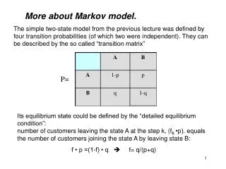
More about Markov model. The simple two-state model from the previous lecture was defined by four transition probabilities (of which two were independent). They can be described by the so called “transition matrix”. P=.

More about Markov model.
E N D
Presentation Transcript
More about Markov model. • The simple two-state model from the previous lecture was defined by four transition probabilities (of which two were independent). They can be described by the so called “transition matrix” P= • Its equilibrium state could be defined by the “detailed equilibrium condition”:number of customers leaving the state A at the step k, (fk•p). equals the number of customers joining the state A by leaving state B: • f • p =(1-f) • q f= q/(p+q)
In general, with s possible states, we can write the transition probability matrix as Any row in this matrix corresponds to the state from which transition is made, and any column corresponds to the state to which transition is made. Thus probabilities in any particular row should sum to 1, while there is no such requirement for the columns (Why? Explain in plain words) . Together with an initial probability distribution, transition matrix determines the Markov process.
Example:Random walks (Evens&Grant, p136: “Random walk theory underpins BLAST theory” The “practical” example involves a gambler ( G) having i dollars and its adversary (A) with (s-i) dollars. At each step a coin with probability p for heads is tossed. If heads come up, A gives G one dollar, and if tails up, then G gives a dollar to A. This continues until the random variable reaches either 0 or s.The random variable is a current fortune of the gambler taking values 0,1,2,…,s dollars. G: 0 1 2 3 s-1 s $
0 dollars 1 dollar 2 dollars s-1 dollar s dollars Example:Random walks (Evens&Grant, p136: “Random walk theory underpins BLAST theory” If G has $1, he throws a coin, and will either gain $1 (probability p) or will lose it (q). He will never stay with $1, and thus p11=0 If G is left without money, he stays in this state with p00=1, and all other transitions become impossible
The transition matrix are widely used in bioinformatics, for sequences analysis. Make sure that you understand why P for the “gambler” has exactly this shape. Why, for instance, p3,5=0? What is the probability of moving from state i to the state j in two steps? We have to sum up the probabilities for all possible “trajectories” connecting i and j. The result is defined by the product P*P of two matrixes (not two numbers!) {m} The product of two matrixes, a and b is the matrix c whose components are j i With this in mind, Eq. 1 can be written as a product Similarly, the n-step transition probability is
0123 1/3 0 1 2 3 1/3 Graphical representation of the Markov Chain Try finding the error
0123 0123 1/6 1/6 1/3 1/3 0 1 2 3 0 1 2 3 1/6 1/3 1/3 1/6 1/6 Graphical representation The corrected diagram
Working in groups: • Find the product of matrixes A and B • open Lect7/Math/Lect7_MatrixExample and use it for practice • Draw a graphical representation for the transition matrixes between the states E1, E2, E3 (a) and E4 (for b) (a) (b)
One application of Markov Model for sequence analysis In the human genome wherever the dinucleotide CG occurs (frequently written CpG to distinguish it from the C-G base pair across the two strands) the C nucleotide (cytosine) is typically chemically modified. There is a relatively high chance of this modification that mutates C into a T, and in general CpG dinucleotides are rarer in the genome than would be expected from the independent probabilities of C and G*. For biologically important reasons the mutation modification process is suppressed in short stretches of the genome, such as around the promoters or ‘start’ regions of many genes. In these regions we see many more CpG dinucleotides than elsewhere. Such regions are called CpG islands. You can find the tool for searching the CpG islands at: http://bioinformatics.org/sms/cpg_island.html • *The CpG dinucleotide is present at approximately 20% of its expected frequency in vertebrate* genomes, a deficiency thought due to a high mutation rate from the methylated form of CpG to TpG and CpA.
What sort of probabilistic model might we use for CpG island regions? It should be a model that generates sequences in which the probability of a symbol depends on the previous symbol. The simplest such model is a classical Markov chain. A Markov chain for DNA can be drawn like this:
where there is a state for each of the four letters A, C, G, and T in the DNA alphabet. The transition probabilities pst are associated with each arrow in the figure and determine the probabilities of a certain residue following another residue (or one “state” following another “state”). Markov models for the CpG island are illustrated below. From a set of human DNA sequences a total of 48 putative CpG islands have been extracted. Two Markov chain models have been developed, one for the regions labeled as CpG islands (the ‘+’ model) and the other from the remainder of the sequence (the ‘-’ model). The transition probabilities for each model were set using the equation
where ctsis the number of times letter t followed letter s in the island regions. These are the maximum likelihood estimators for the transition probabilities. The resulting tables are
The equation (2) therefore becomes Eq. (3) is used to calculate the likelihood of the sequence. For instance, we use (3) to obtain the likelihood values of a sequence under “+” model and “-” model respectively. Comparing them, we can conclude if the sequence belongs to the CpG island region or not. More specifically, we can calculate the log-odds ratio:
A brief introduction to the HMM ·Very efficient programs for searching a text for a combination of words are widely available The same methods can be used for searching for patterns in biological sequences, but often they fail. Why? · Biological ‘spelling’ is much more sloppy than English spelling: proteins with the same function from two different organisms are most likely spelled differently, that is, the two amino acid sequences differ. It is not rare that two such homologous sequences have less than 30% identical amino acids. Similarly in DNA many interesting signals vary greatly even within the same genome. Some well-known examples are ribosome binding sites and splice sites, but the list is long. · Fortunately there are usually still some subtle similarities between two such sequences, and the question is how to detect these similarities.
The variation in a family of sequences can be described statistically, and this is the basis for most methods used in biological sequence analysis • A hidden Markov model (HMM) is a statistical model, which is very well suited for many tasks in molecular biology, although they have been mostly developed for speech recognition since the early 1970s. • The most popular use of the HMM in molecular biology is as a ‘probabilistic profile’ of a protein family, which is called a profile HMM. From a family of proteins (or DNA) a profile HMM can be made for searching a database for other members of the family. • Probably the main contribution of HMM comparative to some other methods is that the profile HMM treats gaps in a systematic way.
From Regular expressions to HMM In programs like grep, JavaScript and Perl, regular expressions can be used for searching text files for a pattern. Using regular expressions is a very elegant and efficient way to search for some protein families, but difficult for other. The difficulties arise because protein spelling is much more free than English spelling. Therefore the regular expressions sometimes need to be very broad and complex. Imagine a DNA motif like this: A regular expression for this is [AT] [CG] [AC] [ACGT]* A [TG] [GC] , meaning that the first position is A or T, the second C or G, and so forth. The term ‘[ACGT]*’ means that any of the four letters can occur any number of times.
The problem with the above regular expression is that it does not in any way distinguish between the highly implausible sequence “TGCT- - AGG” and the consensus sequence “ACAC- -ATC”. It is possible to make the regular expression more discriminative by splitting it into several different ones, but it easily becomes messy. The alternative is to score sequences by how well they fit the alignment.
Such a scoring is shown in the diagram below. This is the HMM derived from the same alignment Transition Probabilities States ‘insertion’ state is represented by the state above the other states.
It is now easy to score the consensus sequence ACACATC. The probabilities of different states (bases) must be multiplied by the transition probabilities: Making the same calculation for the exceptional sequence yieldsonly 0.0023 10-2
Probabilities and log-odds scores for the 5 sequences in the alignment and for the consensus sequence and the ‘exceptional’ sequence:
What is the Log-odds score? The probability itself is not the most convenient number to use as a score, and the log-odds score shown in the last column of the table is usually better. It is the logarithm of the probability of the sequence divided by the probability according to a null model. The null model is one that treats the sequences as random strings of nucleotides, so the probability of a sequence of length L is
The probabilities of the model in the previous picture have been turned into log-odds by taking the logarithm of each nucleotide probability and subtracting log0.25. The transition probabilities have been converted to simple logs. When a sequence fits the motif very well the log-odds is high. When it’s very unlikely, the log-odds score becomes negative. Here is an example for the consensus sequence:
I will stop right here. This discussion was based on a very well-written article (see the “resources” and a link on my site), Reading assignment: pp.8-13 of that article, “Profile HMM” section. This reading will prepare you for better understanding of the project presentation devoted to HMM