GCE Software Tools for Data Mining, Analysis and Synthesis

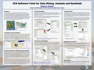
1. Figure 1. U.S. LTER Network sites (left) and real-time USGS stream-flow stations (right) active in 2008 Figure 2. Web-based user interfaces to the GCE-LTER, LTER ClimDB/HydroDB, USGS NWIS and NOAA NWS climate/hydrologic databases GCE Software Tools for Data Mining, Analysis and Synthesis Wade M. SheldonGeorgia Coastal Ecosystems LTER, University of Georgia, Athens, Georgia Integrating Data Sets Several automated and semi-automated tools are also available in the GCE Data Toolbox for integrating multiple data sets for synthesis and comparative analysis. Multiple related data sets (e.g. daily data files for a monitoring station) can be “merged” in one step to create a single time series, with all columns automatically aligned by parameter, data type and units to prevent inappropriate pairings. When data sets that contain overlapping date ranges are merged, records with overlapping dates from the chronologically earlier data set can be automatically trimmed if desired (i.e. to update old records and produce a continuous, monotonic time series). Data sets can also be “joined” by matching values in specified key columns to produce a composite data set containing a mixture of columns selected from both data sets (e.g. air temperature and wind speed from one data set and precipitation from another). Records are automatically aligned according to key column matches to mesh the data set records appropriately. For time-series data sets, key columns for date/time joins can also be identified automatically, greatly simplifying this process (fig.5). Automated Data Retrieval A powerful feature of the GCE Data Toolbox is support for “mining” data from the USGS and LTER databases directly over the Internet, using either interactive graphical dialogs (fig.3) or scriptable command-line functions. Data can be retrieved from any USGS NWIS station or LTER climate site across the country, and browsable lists of stations grouped state/territory (USGS) or by site (LTER) are displayed in data request dialogs for selecting stations. This capability, combined with the metadata templating and QA/QC flagging features, allows users to simultaneously acquire and standardize large amounts of long-term climate and hydrologic data from across the U.S. with just a few mouse clicks or MATLAB commands. Introduction The GCE-LTER project and partner organizations (SINERR, UGAMI, USGS) collect extensive environmental monitoring data around Sapelo Island on the SE Georgia Coast. In order to put these observations into a broader spatial and temporal context, it is also important to compare these data with other environmental monitoring observations. Long-term, spatially-extensive climate and hydrologic databases maintained by the LTER Network (ClimDB/HydroDB), USGS (National Water Information System) and NOAA (National Weather Service) are valuable resources for broad-scale comparisons (fig.1). For example, the LTER Network’s ClimDB/HydroDB database contains approximately 7 million daily records for 281 monitoring stations at 39 LTER and USFS sites, providing critical support for LTER cross-site comparisons. USGS and NOAA collect long-term climate and hydrologic data from a vast array of locations across North America (~8000 real-time USGS monitoring stations and ~12,000 active NWS COOP weather stations), supporting truly large-scale regional analyses. USGS NWIS Data Retrieval Dialog Retrieved Data Set (Editor View) Independent Data Sets Automatic Date/Time Join Dialog Retrieved Data Set (Data View)(note values assigned flags highlighted in red) Plot of Integrated Data (3 Datasets) The Challenge: Dealing with Differences Despite the fact that GCE, other LTER sites, USGS and NOAA all provide free access to long-term data on the World Wide Web (fig.2), obtaining all the data required for a typical synthesis project can be daunting. Finding relevant stations, navigating to data request pages, and choosing data sets and file formatting options require very different procedures on each site. Once data are located and downloaded other challenges arise, such as deciphering different file layouts, harmonizing parameter names and standardizing units. For example, total daily precipitation is variously reported as “Precip (total mm)” in mm from LTER ClimDB, “00045_00006” in inches from USGS, and “Prcp” in inches from NOAA. Conventions for reporting missing values and quality assurance flags also differ among databases. When many data sets are required for an analysis, the cumulative effort required to standardize them can be a limiting factor. Figure 3. Retrieving real-time data from USGS over the Internet and viewing the data using the GCE Data Toolbox (note that data can also be retrieved using command-line functions). A similar dialog is available for retrieving data from the LTER ClimDB/HydroDB database. Figure 5. Automatic date/time join to integrate multiple USGS stream flow datasets for comparison Transforming and Analyzing Data After data sets are acquired and standardized, a wide variety of tools are available for transforming and analyzing the data. Metadata are used to configure dialogs automatically and verify suitability of data selections for each transformation, assuring validity throughout processing. All transformation steps and data set changes are also automatically logged to the metadata to maintain a complete lineage of the data set, which can be reviewed at any time during processing and included in metadata files. Examples of transformations that can be performed: Visualizing Patterns and Trends Several plotting tools are also provided with the GCE Data Toolbox to support data visualization as well as interactive QA/QC flagging with the mouse. A custom zoom toolbar is displayed on data plots to simplify axis scaling and stepping through time-series data sets to identify patterns of interest (fig.6). Plots can be customized and exported in many formats and resolutions for publication, and tools are also provided for automatically generating web pages containing thumbnail views of plots (linked to full-sized plots) at a specified temporal resolution (i.e. daily through decadal time step per plot). unit conversions (interactive and batch English↔Metric) filtering records based on column values or expressions sub-setting data by removing unneeded columns, rows statistical data reduction by aggregation, binning temporal re-sampling (date/time aggregation) (fig.4) generating derived data columns based on expressions splitting compound data series into separate columns The Solution: GCE Tools for Data Mining, Analysis & Synthesis Automating this cumbersome process is clearly necessary to support large-scale data synthesis. At the Georgia Coastal Ecosystems LTER we have developed a suite of MATLAB-based software tools (GCE Data Toolbox for MATLAB) that can help bridge this gap, allowing researchers to acquire, standardize and integrate data from many sources without manual reformatting. These tools can retrieve data from GCE, LTER ClimDB/HydroDB, USGS and NOAA databases directly over the Internet, and also load files downloaded from these program web sites as well as tabular data from a wide variety of other sources (e.g. delimited text files, MATLAB files, data logger files, and SQL database queries). Detailed metadata are automatically generated for each data set using predefined or user-customized templates to standardize column names and provide detailed data type and column units information to support automated analysis. Once data sets are acquired, a wide variety of graphical dialogs and command-line functions can then be used to manipulate, transform, and integrate data sets for analyses and plotting (see below). Powerful rule-based and visual Quality Control tools are also available to identify invalid or questionable values and flag or omit them from subsequent analyses. Data files can also be saved to disk and then indexed, searched and managed using a graphical search engine program distributed with the toolbox. Results from analyses can then be exported in various common formats (plain text, CSV, MATLAB arrays and matrices) for analysis in other data analysis and plotting programs. Experienced MATLAB users can also combine GCE Data Toolbox functions with their own code to automate large-scaled synthesis projects. Figure 6. Left: time series plot of continuous CTD mooring data (note the scroll and zoom buttons at the bottom, and visual QA/QC tools for revising qualifier flags directly on plots). Right: map plot of CTD survey data, illustrating spatial patterns in surface salinity values. 30 minute, real-time data set More Information For more information about the GCE Data Toolbox for MATLAB, or to download the software package (compatible with MATLAB 6.5 or higher, including student versions, running on Windows 2000/XP/Vista, Linux, Solaris and Mac OS/X), visit: http://gce-lter.marsci.uga.edu/public/im/tools/data_toolbox.htm Date/time re-sampling tool Figure 4. Data transformation using the GCE Data Toolbox date/time re-sampling tool. Numbers of flagged and missing values in the source data are automatically tallied in the derived data set, and these tallies can be used to flag statistical results automatically when user-set thresholds for flagged and/or missing values are exceeded. Monthly re-sampled data set