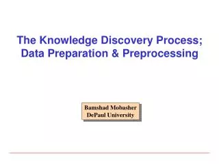
The Knowledge Discovery Process; Data Preparation & Preprocessing
The Knowledge Discovery Process; Data Preparation & Preprocessing. Bamshad Mobasher DePaul University. The Knowledge Discovery Process. - The KDD Process. Types of Data Sets . Record Relational records Data matrix, e.g., numerical matrix, crosstabs

The Knowledge Discovery Process; Data Preparation & Preprocessing
E N D
Presentation Transcript
The Knowledge Discovery Process;Data Preparation & Preprocessing Bamshad Mobasher DePaul University
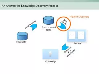
The Knowledge Discovery Process - The KDD Process
Types of Data Sets • Record • Relational records • Data matrix, e.g., numerical matrix, crosstabs • Document data: text documents: term-frequency vector • Transaction data • Graph and network • World Wide Web • Social or information networks • Molecular Structures • Ordered • Video data: sequence of images • Temporal data: time-series • Sequential Data: transaction sequences • Genetic sequence data • Spatial and multimedia: • Spatial data: maps • Image data • Video data
Data Objects • Data sets are made up of data objects. • A data object represents an entity. • Examples: • sales database: object customers, store items, sales • medical database: object patients, treatments • university database: object students, professors, courses • Also called samples , examples, instances, data points, objects, tuples, vectors. • Data objects are described by attributes. • Database rows data objects; columns attributes.
Attributes • Attribute (or dimensions, features, variables): a data field representing a characteristic or property of a data object • E.g., customer _ID, name, address, income, GPA, …. • Types: • Nominal (Categorical) • Ordinal • Numeric: quantitative • Interval-scaled • Ratio-scaled
Attribute Types • Nominal (Categorical): categories, states, or “names of things” • Hair_color = {auburn, black, blond, brown, grey, red, white} • marital status, occupation, ID numbers, zip codes • Often attributes with “yes” and “no” as values • Binary • Nominal attribute with only 2 states (0 and 1) • Ordinal • Values have a meaningful order (ranking) but magnitude between successive values is not known. • Size = {small, medium, large}, grades, army rankings • Month = {jan, feb, mar, … } • Numeric • Quantity (integer or real-valued) • Could also be intervals or ratios
Discrete vs. Continuous Attributes • DiscreteAttribute • Has only a finite or countably infinite set of values • E.g., zip codes, profession, or the set of words in a collection of documents • Sometimes, represented as integer variables • Note: Binary attributes are a special case of discrete attributes • ContinuousAttribute • Has real numbers as attribute values • E.g., temperature, height, or weight • Practically, real values can only be measured and represented using a finite number of digits • Continuous attributes are typically represented as floating-point variables
The Knowledge Discovery Process - The KDD Process
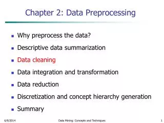
Data Preprocessing • Why do we need to prepare the data? • In real world applications data can be inconsistent, incomplete and/or noisy • Data entry, data transmission, or data collection problems • Discrepancy in naming conventions • Duplicated records • Incomplete or missing data • Contradictions in data • What happens when the data can not be trusted? • Can the decision be trusted? Decision making is jeopardized • Better chance to discover useful knowledge when data is clean
Data Preprocessing Data Cleaning Data Integration Data Transformation -2,32,100,59,48 -0.02,0.32,1.00,0.59,0.48 Data Reduction
Data Cleaning • Real-world application data can be incomplete, noisy, and inconsistent • No recorded values for some attributes • Not considered at time of entry • Random errors • Irrelevant records or fields • Data cleaning attempts to: • Fill in missing values • Smooth out noisy data • Correct inconsistencies • Remove irrelevant data
Dealing with Missing Values • Data is not always available (missing attribute values in records) • equipment malfunction • deleted due to inconsistency or misunderstanding • not considered important at time of data gathering • Solving Missing Data • Ignore the record with missing values; • Fill in the missing values manually; • Use a global constant to fill in missing values (NULL, unknown, etc.); • Use the attribute value mean to filling missing values of that attribute; • Use the attribute mean for all samples belonging to the same class to fill in the missing values; • Infer the most probable value to fill in the missing value • may need to use methods such as Bayesian classification or decision trees to automatically infer missing attribute values
Smoothing Noisy Data • The purpose of data smoothing is to eliminate noise and “smooth out” the data fluctuations. Ex: Original Data for “price” (after sorting): 4, 8, 15, 21, 21, 24, 25, 28, 34 Partition into equidepth bins Bin1: 4, 8, 15 Bin2: 21, 21, 24 Bin3: 25, 28, 34 Binning Min and Max values in each bin are identified (boundaries). Each value in a bin is replaced with the closest boundary value. Each value in a bin is replaced by the mean value of the bin. means Bin1: 9, 9, 9 Bin2: 22, 22, 22 Bin3: 29, 29, 29 boundaries Bin1: 4, 4, 15 Bin2: 21, 21, 24 Bin3: 25, 25, 34
Smoothing Noisy Data • Other Methods Similar values are organized into groups (clusters). Values falling outside of clusters may be considered “outliers” and may be candidates for elimination. Clustering Fit data to a function. Linear regression finds the best line to fit two variables. Multiple regression can handle multiple variables. The values given by the function are used instead of the original values. Regression
Smoothing Noisy Data - Example • Want to smooth “Temperature” by bin means with bins of size 3: • First sort the values of the attribute (keep track of the ID or key so that the transformed values can be replaced in the original table. • Divide the data into bins of size 3 (or less in case of last bin). • Convert the values in each bin to the mean value for that bin • Put the resulting values into the original table
Smoothing Noisy Data - Example Value of every record in each bin is changed to the mean value for that bin. If it is necessary to keep the value as an integer, then the mean values are rounded to the nearest integer.
Smoothing Noisy Data - Example The final table with the new values for the Temperature attribute.
Data Integration • Data analysis may require a combination of data from multiple sources into a coherent data store • Challenges in Data Integration: • Schema integration: CID = C_number = Cust-id = cust# • Semantic heterogeneity • Data value conflicts (different representations or scales, etc.) • Synchronization (especially important in Web usage mining) • Redundant attributes (redundant if it can be derived from other attributes) -- may be able to identify redundancies via correlation analysis: • Meta-data is often necessary for successful data integration Pr(A,B) / (Pr(A).Pr(B)) = 1: independent, > 1: positive correlation, < 1: negative correlation.
Data Transformation: Normalization • Min-max normalization: linear transformation from v to v’ • v’ = [(v - min)/(max - min)] x (newmax - newmin) + newmin • Note that if the new range is [0..1], then this simplifies to v’ = [(v - min)/(max - min)] • Ex: transform $30000 between [10000..45000] into [0..1] ==> [(30000 – 10000) / 35000] = 0.514 • z-score normalization: normalization of v into v’ based on attribute value mean and standard deviation • v’ = (v - Mean) / StandardDeviation • Normalization by decimal scaling • moves the decimal point of v by j positions such that j is the minimum number of positions moved so that absolute maximum value falls in [0..1]. • v’ = v / 10j • Ex: if v in [-56 .. 9976] and j=4 ==> v’ in [-0.0056 .. 0.9976]
Normalization: Example • z-score normalization: v’ = (v - Mean) / Stdev • Example: normalizing the “Humidity” attribute: Mean = 80.3 Stdev = 9.84
Normalization: Example II • Min-Max normalization on an employee database • max distance for salary: 100000-19000 = 81000 • max distance for age: 52-27 = 25 • New min for age and salary = 0; new max for age and salary = 1
Data Transformation: Discretization • 3 Types of attributes • nominal - values from an unordered set (also “categorical” attributes) • ordinal - values from an ordered set • numeric/continuous- real numbers (but sometimes also integer values) • Discretization is used to reduce the number of values for a given continuous attribute • usually done by dividing the range of the attribute into intervals • interval labels are then used to replace actual data values • Some data mining algorithms only accept categorical attributes and cannot handle a range of continuous attribute value • Discretization can also be used to generate concept hierarchies • reduce the data by collecting and replacing low level concepts (e.g., numeric values for “age”) by higher level concepts (e.g., “young”, “middle aged”, “old”)
Discretization - Example • Example: discretizing the “Humidity” attribute using 3 bins. Low = 60-69 Normal = 70-79 High = 80+
Data Discretization Methods • Binning • Top-down split, unsupervised • Histogram analysis • Top-down split, unsupervised • Clustering analysis • Unsupervised, top-down split or bottom-up merge • Decision-tree analysis • Supervised, top-down split • Correlation (e.g., 2) analysis • Unsupervised, bottom-up merge 25
Simple Discretization: Binning • Equal-width (distance) partitioning • Divides the range into N intervals of equal size: uniform grid • if A and B are the lowest and highest values of the attribute, the width of intervals will be: W = (B –A)/N. • The most straightforward, but outliers may dominate presentation • Skewed data is not handled well • Equal-depth (frequency) partitioning • Divides the range into N intervals, each containing approximately same number of samples • Good data scaling • Managing categorical attributes can be tricky
Discretization Without Using Class Labels(Binning vs. Clustering) Data Equal interval width (binning) Equal frequency (binning) K-means clustering leads to better results 27
Discretization by Classification & Correlation Analysis • Classification (e.g., decision tree analysis) • Supervised: Given class labels, e.g., cancerous vs. benign • Using entropy to determine split point (discretization point) • Top-down, recursive split • Correlation analysis (e.g., Chi-merge: χ2-based discretization) • Supervised: use class information • Bottom-up merge: merge the best neighboring intervals (those with similar distributions of classes, i.e., low χ2 values) • Merge performed recursively, until a predefined stopping condition 28
Converting Categorical Attributes to Numerical Attributes Attributes: Outlook (overcast, rain, sunny) Temperature real Humidity real Windy (true, false) Standard Spreadsheet Format Create separate columns for each value of a categorical attribute (e.g., 3 values for the Outlook attribute and two values of the Windy attribute). There is no change to the numerical attributes.
Data Reduction • Data is often too large; reducing data can improve performance • Data reduction consists of reducing the representation of the data set while producing the same (or almost the same) results • Data reduction includes: • Data cube aggregation • Dimensionality reduction • Discretization • Numerosity reduction • Regression • Histograms • Clustering • Sampling
Data Cube Aggregation • Reduce the data to the concept level needed in the analysis • Use the smallest (most detailed) level necessary to solve the problem • Queries regarding aggregated information should be answered using data cube when possible
Dimensionality Reduction • Curse of dimensionality • When dimensionality increases, data becomes increasingly sparse • Density and distance between points, which is critical to clustering, outlier analysis, becomes less meaningful • The possible combinations of subspaces will grow exponentially • Dimensionality reduction • Avoid the curse of dimensionality • Help eliminate irrelevant features and reduce noise • Reduce time and space required in data mining • Allow easier visualization • Dimensionality reduction techniques • Principal Component Analysis • Attribute subset selection • Attribute or feature generation
Principal Component Analysis (PCA) • Find a projection that captures the largest amount of variation in data • The original data are projected onto a much smaller space, resulting in dimensionality reduction • Done by finding the eigenvectors of the covariance matrix, and these eigenvectors define the new space x2 e x1
Principal Component Analysis (Steps) • Given N data vectors (rows in a table) from ndimensions (attributes), find k ≤ n orthogonal vectors (principal components) that can be best used to represent data • Normalize input data: Each attribute falls within the same range • Compute k orthonormal (unit) vectors, i.e., principal components • Each input data (vector) is a linear combination of the k principal component vectors • The principal components are sorted in order of decreasing “significance” or strength • The size of the data can be reduced by eliminating the weak components, i.e., those with low variance • Using the strongest principal components, it is possible to reconstruct a good approximation of the original data • Works for numeric data only
Attribute Subset Selection • Another way to reduce dimensionality of data • Redundant attributes • Duplicate much or all of the information contained in one or more other attributes • E.g., purchase price of a product and the amount of sales tax paid • Irrelevant attributes • Contain no information that is useful for the data mining task at hand • E.g., students' ID is often irrelevant to the task of predicting students' GPA
Heuristic Search in Attribute Selection • There are 2d possible attribute combinations of d attributes • Typical heuristic attribute selection methods: • Best single attribute under the attribute independence assumption: choose by significance tests • Best step-wise feature selection: • The best single-attribute is picked first. Then next best attribute condition to the first, ... • {}{A1}{A1, A3}{A1, A3, A5} • Step-wise attribute elimination: • Repeatedly eliminate the worst attribute: {A1, A2, A3, A4, A5}{A1, A3, A4, A5} {A1, A3, A5}, …. • Combined attribute selection and elimination • Decision Tree Induction
Decision Tree Induction Use information theoretic techniques to select the most “informative” attributes
Attribute Creation (Feature Generation) • Create new attributes (features) that can capture the important information in a data set more effectively than the original ones • Three general methodologies • Attribute extraction • Domain-specific • Mapping data to new space (see: data reduction) • E.g., Fourier transformation, wavelet transformation, etc. • Attribute construction • Combining features • Data discretization 38
Data Reduction: Numerosity Reduction • Reduce data volume by choosing alternative, smaller forms of data representation • Parametric methods (e.g., regression) • Assume the data fits some model, estimate model parameters, store only the parameters, and discard the data (except possible outliers) • Ex.: Log-linear models—obtain value at a point in m-D space as the product on appropriate marginal subspaces • Non-parametric methods • Do not assume models • Major families: histograms, clustering, sampling, …
Collection of techniques for the modeling and analysis of numerical data consisting of values of a dependent variable (also response variable or measurement) and of one or more independent variables (aka. explanatory variables or predictors) The parameters are estimated to obtains a "best fit" of the data Typically the best fit is evaluated by using the least squares method, but other criteria have also been used Used for prediction (including forecasting of time-series data), inference, hypothesis testing, and modeling of causal relationships Y1 Y1’ y = x + 1 x X1 Regression Analysis y
Regression Analysis • Linear regression: Y = w X + b • Two regression coefficients, w and b, specify the line and are to be estimated by using the data at hand • Using the least squares criterion on known values of Y1, Y2, …, X1, X2, …. • Multiple regression: Y = b0 + b1 X1 + b2 X2 • Many nonlinear functions can be transformed into the above • Log-linear models • Approximate discrete multidimensional probability distributions • Estimate the probability of each point in a multi-dimensional space for a set of discretized attributes, based on a smaller subset of dimensions • Useful for dimensionality reduction and data smoothing
Numerocity Reduction • Reduction via histograms: • Divide data into buckets and store representation of buckets (sum, count, etc.) • Reduction via clustering • Partition data into clusters based on “closeness” in space • Retain representatives of clusters (centroids) and outliers • Reduction via sampling • Will the patterns in the sample represent the patterns in the data? • Random sampling can produce poor results • Stratified sample (stratum = group based on attribute value)
Sampling Techniques SRSWOR (simple random sample without replacement) SRSWR Raw Data Cluster/Stratified Sample Raw Data