Voice DSP Processing II
Voice DSP Processing II. Yaakov J. Stein Chief Scientist RAD Data Communications. Voice DSP. Part 1 Speech biology and what we can learn from it Part 2 Speech DSP (AGC, VAD, features, echo cancellation) Part 3 Speech compression techiques Part 4 Speech Recognition.

Voice DSP Processing II
E N D
Presentation Transcript
VoiceDSPProcessingII Yaakov J. Stein Chief ScientistRAD Data Communications
Voice DSP Part 1 Speech biology and what we can learn from it Part 2 Speech DSP (AGC, VAD, features, echo cancellation) Part 3 Speech compression techiques Part 4 Speech Recognition
Voice DSP - Part 2 Simplest processing • Gain • AGC • VAD More complex processing • pitch tracking • U/V decision • computing LPC • other features • Echo Cancellation • Sources of echo • Echo suppression • Echo cancellation • Adaptive noise cancellation • The LMS algorithm • Other adaptive algorithms • The standard LEC
Voice DSP - Part 2a Simplest voice DSP
Gain (volume) Control In analog processing (electronics) gain requires an amplifier Great care must be taken to ensure linearity! In digital processing (DSP) gain requires only multiplication y = G x Need enough bits!
Automatic Gain Control (AGC) Can we set the gain automatically? Yes, based on the signal’s Energy! E = x2 (t) dt = S xn2 All we have to do is apply gain until attain desired energy Assume we want the energy to be Y Then y = Y/ E x = G x has exactly this energy
AGC - cont. What if the input isn’t stationary (gets stronger and weaker over time) ? The energy is defined for all times- < t < so it can’t help! So we define “energy in window” E(t) and continuously vary gain G(t) This is Adaptive Gain Control We don’t want gain to jump from window to window so we smooth the instantaneous gain G(t)a G(t) + (1-a) Y/E(t) IIR filter 8 8
AGC - cont. Theacoefficient determines how fastG(t)can change In more complex implementations we may separately control integration time, attack time, release time What is involved in the computation ofG(t)? • Squaring of input value • Accumulation • Square root (or Pythagorean sum) • Inversion (division) Square root and inversion are hard for a DSP processor but algorithmic improvements are possible (and often needed)
Simple VAD Sometimes it is useful to know whether someone is talking (or not) • Save bandwidth • Suppress echo • Segment utterances We might be able to get away with “energy VOX” Normally need Noise Riding Threshold / Signal Riding Threshold However, there are problems energy VOX since it doesn’t differentiate between speech and noise What we really want is a speech-specific activity detector Voice Activity Detector
Simple VAD - cont. VADs operate by recognizing that speech is different from noise • Speech is low-pass while noise is white • Speech is mostly voiced and so has pitch in a given range • Average noise amplitude is relatively constant A simple VAD may use: • zero crossings • zero crossing “derivative” • spectral tilt filter • energy contours • combinations of the above
Other “simple” processes Simple = not significantly dependent on details of speech signal • Speed change of recorded signal • Speed change with pitch compensation • Pitch change with speed compensation • Sample rate conversion • Tone generation • Tone detection • Dual tone generation • Dual tone detection (need high reliability)
Voice DSP - Part 2b Complex voice DSP
Correlation One major difference between simple and complex processing is the computation of correlations (related to LPC model) Correlation is a measure of similarity Shouldn’t we use squared difference to measure similarity? D2 = < (x(t) - y(t))2> No, since squared difference is sensitive to • gain • time shifts
Correlation - cont. D2 = < (x(t) - y(t))2>= < x2 > + < y2 > - 2 <x(t) y(t)> So whenD2 is minimal C(0) = <x(t) y(t)> is maximal and arbitrary gains don’t change this To take time shifts into account C(t) = <x(t) y(t+t)> and look for maximal t ! We can even find out how much a signal resembles itself
Autocorrelation CrosscorrelationCx y (t) = <x(t) y(t+t)> AutocorrelationCx (t) = <x(t) x(t+t)> Cx (0) is the energy! Autocorrelation helps find hidden periodicities! Much stronger than looking in the time representation Wiener Khintchine Autocorrelation C(t) and Power Spectrum S(f) are FT pair So autocorrelation contains the same information as the power spectrum … and can itself be computed by FFT
Pitch tracking How can we measure (and track) the pitch? We can look for it in the spectrum • but it may be very weak • may not even be there (filtered out) • need high resolution spectral estimation Correlation based methods The pitch periodicity should be seen in the autocorrelation! Sometimes computationally simpler is the Absolute Magnitude Difference Function < | x(t) - x(t+t) |>
Pitch tracking - cont. Sondhi’s algorithm for autocorrelation-based pitch tracking : • obtain window of speech • determine if the segment is voiced (see U/V decision below) • low-pass filter and center-clip to reduce formant induced correlations • compute autocorrelation lags corresponding to valid pitch intervals • find lag with maximum correlation OR • find lag with maximal accumulated correlation in all multiples Post processing Pitch trackers rarely makesmallerrors(usually double pitch) So correct outliers based on neighboring values
Other Pitch Trackers Miller’s data-reduction& Gold and Rabiner’s parallel processing methods Zero-crossings, energy, extrema of waveform Noll’s cepstrum based pitch tracker Since the pitch and formant contributions are separated in cepstral domain Most accurate for clean speech, but not robust in noise Methods based on LPC error signal LPC technique breaks down at pitch pulse onset Find periodicity of error by autocorrelation Inverse filtering method Remove formant filtering by low-order LPC analysis Find periodicity of excitation by autocorrelation Sondhi-like methods are the best for noisy speech
U/V decision Between VAD and pitch tracking • Simplest U/V decision is based on energy and zero crossings • More complex methods are combined with pitch tracking • Methods based on pattern recognition Is voicing well defined? • Degree of voicing (buzz) • Voicing per frequency band (interference) • Degree of voicing per frequency band
LPC Coefficients How do we find the vocal tract filter coefficients? System identification problem • All-pole (AR) filter • Connection to prediction Sn = G en+ Sm am sn-m Can find G from energy (so let’s ignore it) Unknown filter known input known output
LPC Coefficients For simplicity let’s assume threeacoefficients Sn = en+ a1 sn-1 + a 2 s n-2 + a 3 s n-3 Need three equations! Sn= en+ a1 sn-1 + a 2 s n-2 + a 3 s n-3 Sn+1 = en+1+ a1 sn+ a 2 s n-1 + a 3 s n-2 Sn+2 = en+2+ a1 sn+1 + a 2 s n + a 3 s n-1 In matrix form Snensn-1 s n-2 s n-3a1 Sn+1 = en+1+ sns n-1 s n-2a 2 Sn+2 en+2sn+1 s n s n-1a 3 s = e + S a
LPC Coefficients - cont. S = e + S a so by simple algebra a = S-1 ( s - e ) and we have reduced the problem to matrix inversion Toeplitz matrix so the inversion is easy (Levinson-Durbin algorithm) Unfortunately noise makes this attempt break down! Move to next time and the answer will be different. Need to somehow average the answers The proper averaging is before the equation solving correlation vs autocovariance
LPC Coefficients - cont. Can’t just average over time - all equations would be the same! Let’s take the input to be zero Sn = Sm am sn-m multiply bySn-q and sum over n Sn Sn Sn-q = Sm am Sn sn-msn-q we recognize the autocorrelations Cs (q) = SmCs (|m-q|) am Yule-Walker equations autocorrelation method: sn outside window are zero (Toeplitz) autocovariance method: use all needed sn (no window) Also - pre-emphasis!
Alternative features The a coefficients aren’t the only set of features • Reflection coefficients (cylinder model) • log-area coefficients (cylinder model) • pole locations • LPC cepstrum coefficients • Line Spectral Pairfrequencies All theoretically contain the same information (algebraic transformations) • Euclidean distance in LPC cepstrum space ~ Itakura Saito measure so these are popular in speech recognition • LPC (a) coefficients don’t quantize or interpolate well so these aren’t good for speech compression • LSP frequencies are best for compression
LSP coefficients • a coefficients are not statistically equally weighted • pole positions are better (geometric) but radius is sensitive near unit circle • Is there an all-angle representation? Theorem 1: Every real polynomial with all roots on the unit circle is palindromic (e.g. 1 + 2t + t2) or antipalindromic (e.g. t + t2 - t3) Theorem 2: Every polynomial can be written as the sum of palindromic and antipalindromic polynomials Consequence: Every polynomial can be represented by roots on the unit circle, that is,by angles
Voice DSP - Part 2c Echo Cancellation
Line echo hybrid hybrid Telephone 1 Telephone 2
4w switch comp inv 4w switch Echo suppressor In practice need more: VOX, over-ride, reset, etc.
- near end far end Why not echo suppresion? • Echo suppression makes conversation half duplex • Waste of full-duplex infrastructure • Conversation unnatural • Hard to break in • Dead sounding line It would be better to cancel the echo subtract the echo signal allowing desired signal through but that requires DSP.
clean Echo cancellation? Unfortunately, it’s not so easy Outgoing signal is delayed, attenuated, distorted Two echo canceller architectures: MODEM TYPE LINE ECHO CANCELLER (LEC) - echo path near end far end clean clean - near end far end echo path
LEC architecture h y b r i d A/D NLP - Y filter H doubletalk detector adapt near end far end X D/A
Adaptive Algorithms How do we • find the echo cancelling filter? • keep it correct even if the echo path parameters change? Need an algorithm that continually changes the filter parameters All adaptive algorithms are based on the same ideas (lack of corellation between desired signal and interference) Let’s start with a simpler case - adaptive noise cancellation
Noise cancellation y h n x e n y x - n h e
Noise cancellation - cont. Assume that noise is distorted only by unknown gain h We correct by transmitting e n so that the audience hears y = x + h n - e n = x + (h-e) n the energy of this signal is Ey = < y2 > = < x2> + (h-e)2< n2> + 2(h-e) < x n> Assume that Cxn = < x n> = 0 We need only seteto minimize Ey ! (turn knob until minimal) Even if the distortion is a complete filter h we set the ANC filter e to minimize Ey
The LMS algorithm Gradient descent on energy correction to H is proportional to error d times input X H H + l d X
Nonlinear processing Because of finite numeric precision the LEC (linear) filtering can not completely remove echo Standard LEC adds center clipping to remove residual echo Clipping threshold needs to be properly set by adaptation
Doubletalk detection Adaptation of H should take place only when far end speaks So we freeze adaptation when no far end or double-talk, that is whenever near end speaks Geigel algorithm compares absolute value of near-end speech to half the maximum absolute value in X buffer If near-end exceeds far-end can assume only near-end is speaking