Download
1 / 42
420 likes | 585 Views
Petascale astronomy and the SKA. Athol Kemball Department of Astronomy & Center for Extreme-scale Computing (IACAT/NCSA) University of Illinois, USA akemball@illinois.edu. Contemporary scientific methods. Euclid, 3 rd century mathematician, teaching ( Raphael). Theory:

E N D
Petascale astronomy and the SKA Athol Kemball Department of Astronomy & Center for Extreme-scale Computing (IACAT/NCSA) University of Illinois, USA akemball@illinois.edu
Contemporary scientific methods Euclid, 3rd century mathematician, teaching (Raphael) • Theory: • Develop abstract or mathematical models of the physical system or problem. • Experimental and observational methods: • Take observational or experimental data to disprove or refine models • Computational methods: • Simulate complex multi-scale systems that are beyond the reach of analytic methods • Process vast amounts of observed or experiment data Very Large Array (VLA); New Mexico, USA Molecular dynamics simulation: water permeation in aquaporins (Schulten Group, UIUC
Computational Cosmology: Structure Formation Nonlinear Evolution of the Universe:from 20 million to 14 billion years old The cosmological simulation computes the nonlinear evolution of the universe in the context of the standard cosmological model determined by the Wilkinson Microwave Background Anisotropy experiment. (Cen & Ostriker 2006; Advanced Vizualization Laboratory NCSA)
Computational Science: Ensuring …President’s Information Technology Advisory Committee “Together with theory and experiment, computational science now constitutes the “third pillar” of scientific inquiry, enabling researchers to build and test models of complex phenomena – such as multi-century climate shifts, multidimensional flight stress on aircraft, and stellar explosions – that cannot be replicated in the laboratory, and to manage huge volumes of data rapidly and economically.” While it is itself a discipline, computational science serves to advance all of science. The most scientifically important and economically promising research frontiers in the 21st century will be conquered by those most skilled with advanced computing technologies and computational science applications.”
Computational Science and Engineering Molecular Science Weather & Climate Forecasting Health Astronomy Earth Science
Fundamental questions in physics and astronomy “What are the basic properties of the fundamental particles and forces?” Neutrinos, Magnetic Fields, Gravity, Gravitational Waves, Dark Energy “What constitutes the missing mass of the Universe?” Cold Dark Matter (e.g. via lensing), Dark Energy, Hot Dark Matter (neutrinos) “What is the origin of the Universe and the observed structure and how did it evolve?” Atomic hydrogen, epoch of reionization, magnetic fields, star-formation history…… “How do planetary systems form and evolve?” Movies of Planet Formation, Astrobiology, Radio flares from exo-planets…… “Has life existed elsewhere in the Universe, and does it exist elsewhere now?” SETI
How does SKA answer these questions ? • Detect and image neutral hydrogen in the very early phases of the universe when the first stars and galaxies appeared “epoch of re-ionization” • Locate 1 billion galaxies via their neutral hydrogen signature and measure their distribution in space – “dark energy”
How does SKA answer these questions ? • Time pulsars to test description of gravity in the strong field case (pulsar-Black Hole binaries), and to detect gravitational waves; explore the unknown transient universe • Origin and evolution of cosmic magnetic fields – “the magnetic universe” • Planet formation – image Earth-sized gaps in proto-planetary disks BLACK HOLE
The Large Synoptic Survey Telescope (2014) LSST science goals • Cosmology: probing dark energy and dark matter • Exploring the transient sky • Mapping the Milky Way • Inventory of Solar System objects (LSST; 8.4m; 3.2 Gpixel camera) (LSST deep lensing survey (Ivezic et al. 2008)) (Cerro Panchon (Iveziv et al. 2008))
The Great Survey Era SKA-era telescopes & science require: • Surveys over large cosmic volumes (Ω,z), fine synoptic time-sampling Δt, and/or high completeness • High receptor count and data acquisition rates • Software/hardware boundary far closer to receptors than at present • Efficient, high-throughput survey operations modes Processing implications • High sensitivity, Ae/Tsys~104 m2K-1, wide-field imaging; • Demanding (t,ω,P) non-imaging analysis • Large O(109) survey catalogs High associated data rates (TBps), compute processing rates (PF), and PB/EB archives (SKA schematic: tiled aperture arrays plus parabolic dishes) (HI galaxy surveys, e.g. ALFALFA HI (Giovanelli et al. 2007); SKA requires a billion galaxy survey.)
LSST computing and data storage scale Reference science requires: • Telescope data output of 15 TB per night • Archive size ~ O(102) PB • Processing ~ O(1) PF (LSST data flow (Ivezic et al. 2008)) 14 (LSST focal plan: each square 4k x 4k pixels; (Ivezic et al. 2008))
SKA wide-field image formation Algorithm technologies • 3-D transform (Perley 1999), facet-based tesselation / polyhedral imaging (Cornwell & Perley 1992), and w-projection (Cornwell et al. 2003). (Cornwell et al. 2003; facet-based vs w-projection algorithms)
SKA computing and data scale • LNSD data rates (Perley & Cornwell 2003): where D = dish diameter, B = max. baseline, Δν = bandwidth, and ν = frequency • Wide-field imaging cost ~ O(D-4 to -8) (Perley & Clark 2003; Cornwell 2004; Lonsdale et al 2004). • Full-field continuum imaging cost (derived from Cornwell 2004): • Strong dependence on 1/Dand B. Data rates of Tbps and computational costs in PF are readily obtained from underlying geometric terms. • Spectral line imaging costs exceed continuum imaging costs. • Possible mitigation through FOV tailoring (Lonsdale et al 2004), beam-forming, and antenna aggregation approaches (Wright et al.) • 550 GBps/na2 (Lonsdale et al 2004) • Runaway petascale costs for SKA tightly coupled to design choices
Commoditization effects in computing hardware costs models for general- purpose CPU and GPU accelerators at a fixed epoch (2007). Estimated from public data. The declining cost of high-performance computing hardware • Computing hardware system costs vary over key primary axes: • Time evolution (Moore’s Law) • Level of commoditization Moore’s Law for general-purpose Intel CPUs. Trend-line for Top 500 leading-edge performance.
Computing hardware performance and cost models • Predicted leading-edge LINPACK Rmax performance from Top 500 trend-line (from data tyr = [1993, 2007]): • Cost per unit teraflop cTF(t), for a commiditzation factor η, Moore’s Law doubling time Δt, and construction lead time Δc: [with cTF(t0) = $300k/TF, t0 = 2007, η = [0.3-1.0], Δt ~ 1.5 yr, Δc ~ 1-4 yr]
Directions in Computing TechnologyIncreasing Clock Frequency & Performance “In the past, performance scaling in conventional single-core processors has been accomplished largely through increases in clock frequency (accounting forroughly 80 percent of the performance gains to date).” Platform 2015 S. Y. Borkar et al., 2006 Intel Corporation Frequency (MHz) Intel Pentium
Directions in Computing TechnologyProblem with Uni-core Microprocessors Rocket Nozzle 1000 Nuclear Reactor Pentium 4 (Prescott) 100 Pentium 4 (Willamette) Watts/cm2 Pentium III Hot Plate Pentium II 10 Pentium Pro Pentium i386 i486 1 1.5m 1.0m 0.7m 0.5m 0.35m 0.25m 0.18m 0.13m 0.1m 0.07m Decreasing Feature Size Increasing Chip Frequency
Directions in Computing TechnologyFrom Uni-core to Multi-core Processors AMD Uni-, Dual-, Quad-core, Processors Intel Teraflops Chip Intel Multi-core Performance
Directions in Computing TechnologySwitch to Multicore Chips “For the next several years the only way to obtain significant increases in performance will be through increasing use of parallelism: – 4× now – 8× in 2009 – 16× in 2011 – … dual core quad core Frequency (MHz)
Trends at extreme scale Inconvenient truths • Moore’s Law holds, but high-performance architectures are evolving rapidly: • Breakpoint in clock speed evolution (2004) • Lateral expansion to multi-core processors and processor augmentation with accelerators • Theoretical performance ≠ actual performance • Sustained petascale calibration and imaging performance for SKA requires: • Demonstrated mapping of SKA calibration and imaging algorithms to modern HPC architectures, and proof of feasible scalability to petascale: [O(105) processor cores]. • Remains a considerable design unknown in both feasibility and cost. (Golap, Kemball et al. 2001, Coma cluster, VLA 74 MHz, parallelized facet-based wide-field imaging)
Scalability *Abe: Dell 1955 blade cluster – 2.33 GHz Intel Cloverton Quad-Core • 1,200 blades/9,600 cores • 89.5 TF; 9.6 TB RAM; 170 TB disk – Power/Cooling • 500 KW / 140 tons (Dunning 2007)
Challenges and Solutions in Petascale Computing Petascale Computing Facility Partners EYP MCF/ Gensler IBM Yahoo! • Energy Efficiency • LEED certified (goal: silver) • Efficient cooling system • Modern Data Center • 90,000+ ft2 total • 20,000 ft2 machine room www.ncsa.uiuc.edu/BlueWaters
Innovative Computing TechnologiesOn to Many-core Chips NVIDIA GeForce 8800 GTX (128 cores) IBM Cell (1+8 cores) Intel Teraflops Chip (80 cores)
NVIDIA (GPU) INTEL (CPU) Innovative Computing TechnologiesNew Technologies for Petascale Computing 400 1.50 GHz G80 350 1.35 GHz G80 300 250 Gflops 200 150 2.66 GHz Quad-core 100 3.4 GHz Dual-core 50 0 2002 2003 2004 2005 2006 2007 Courtesy of John Owens (UCSD) & Ian Buck (NVIDIA)
Texture Texture Texture Texture Texture Texture Texture Texture Texture Host Input Assembler Thread Execution Manager Parallel DataCache Parallel DataCache Parallel DataCache Parallel DataCache Parallel DataCache Parallel DataCache Parallel DataCache Parallel DataCache Load/store Load/store Load/store Load/store Load/store Load/store Global Memory Innovative Computing TechnologiesNVIDIA: GeForce 8800 GTX GPU 128 Cores, 346 GFLOPS (SP), 768 MB DRAM, 86.4 GB/s memory bandwidth; CUDA* * Compute Unified Device Architecture
Innovative Computing TechnologiesNVIDIA: Selected Benchmarks * W-m. Hwu et al., 2007
Feasibility: imaging dynamic range Reference specifications (Schillizzi et al 2007) • Targeted λ20cm continuum field: 107:1. • Routine λ20cm continuum: 106:1. • Driven by need to achieve thermal noise limit (nJy) over plausible field integrations. • Spectral dynamic range: 105:1. • Current typical state of practice near λ ~ 20 cm given below. (de Bruyn and Brentjens, 2005) High-sensitivity deep fields Dynamic range
Image-plane calibration effect Visibility on baseline m-n Source brightness (I,Q,U,V) Direction on sky: ρ Feasibility: imaging dynamic range Basic imaging and calibration equation for radio interferometry (e.g. Hamaker, Bregman, & Sault et al.): Visibility-plane calibration effect Key challenges • Robust, high-fidelity image-plane (ρ) calibration: • Non-isoplanatism. • Antenna pointing errors. • Polarized beam response in (t,ω), … • Non-linearities, non-closing errors • Deconvolution and sky model limits • Dynamic range budget will be set by system design elements. (Bhatnagar et al. 2004; antenna pointing self-cal: 12µJy => 1µJy rms)
Image-plane calibration effect Visibility on baseline m-n Source brightness (I,Q,U,V) Direction on sky: ρ Feasibility: imaging dynamic range Basic imaging and calibration equation for radio interferometry (e.g. Hamaker, Bregman, & Sault et al.): Visibility-plane calibration effect Calibration challenges • Number of free parameters in image-plane terms far greater than visibility-plane terms: • Requires large-parameter solvers for multiple calibration terms • Stability, robustness, and convergence an open research topic. • Large-N arrays will almost certainly operated with reference Global Sky Models (GSM) • As well-calibrated as possible in routine observing. • A new paradigm, however … • Pathfinders will inject reality here
Feasibility: dynamic range assessment SKA dynamic range assessment – beyond the central pixel • Current achieved dynamic ranges degrade significantly with radial projected distance from field center, for reasons understood qualitatively (e.g. direction-dependent gains, sidelobe confusion etc.) • An SKA design with routine uniform, ultra-high dynamic range requires a quantitative dynamic range budget. • Strategies: • Real data from similar pathfinders (e.g. MeerKAT) are key. • Simulations are useful if relative dynamic range contributions or absolute fidelity are being assessed with simple models. • Newstatistical methods: • Assume convergent, regularized imaging estimator for brightness distribution within imaging equation; need to know sampling distribution of imaging estimator per pixel, but unknown PDF a priori: • Statistical resampling (Kemball & Martinsek 2005ff) and Bayesian methods (Sutton & Wandeldt 2005) offer new approaches.
Truth from MC simulation Other estimates from statistical methods Direction-dependent variance estimation methods (Kemball et al. (2008), AJ)
Software cost models • Computer operations costs: ~ 10% of system construction costs p.a. • Software development costs (Boehm et al. 1981): where β ~ ratio of academic to commerical software construction costs. • LSST computing costs approximately one quarter of project; order of magnitude smaller data rates than SKA (~ tens of TB per night); total construction costs perhaps a third of SKA. (LSST)
Approaching the SKA petascale challenges • Form interdisciplinary institutes and teams: • Computer scientists, computer engineers, and applications scientists • Invest in people not hardware • Develop international projects and collaborations • Focus on the (multi-wavelength) science goals • Revisit current imaging algorithms for extreme scalability • Learn from other disciplines in the physical sciences preparing for the petascale era • New sociology needed concerning observing and data practices
Great Lakes Consortium for Petascale Computation Goal: Facilitate the widespread and effective use of petascale computing to address frontier research questions in science, technology and engineering at research, educational and industrial organizations across the region and nation. Charter Members Argonne National Laboratory Fermi National Accelerator Laboratory Illinois Math and Science Academy Illinois Wesleyan University Indiana University* Iowa State University Illinois Mathematics and Science Academy Krell Institute, Inc. Louisiana State University Michigan State University* Northwestern University* Parkland Community College Pennsylvania State University* Purdue University* The Ohio State University* Shiloh Community Unit School District #1 Shodor Education Foundation, Inc. SURA – 60 plus universities University of Chicago* University of Illinois at Chicago* University of Illinois at Urbana-Champaign* University of Iowa* University of Michigan* University of Minnesota* University of North Carolina–Chapel Hill University of Wisconsin–Madison* Wayne City High School * CIC universities*
. Calgary . . . Cornell . . MIT UIUC UCB . UNM NRL NRAO US SKA calibration & processing working group (TDP) • Athol Kemball (Illinois) (Chair) • Sanjay Bhatnagar (NRAO) • Geoff Bower (UCB) • Jim Cordes (Cornell; TDP PI) • Shep Doeleman (Haystack/MIT) • Joe Lazio (NRL) • Colin Lonsdale (Haystack/MIT) • Lynn Matthews (Haystack/MIT) • Steve Myers (NRAO) • Jeroen Stil (Calgary) • Greg Taylor (UNM) • David Whysong (UCB)
Approaching the SKA petascale challenges • Form interdisciplinary institutes and teams: • Computer scientists, computer engineers, and applications scientists • Invest in people not hardware • Develop international projects and collaborations • Focus on the (multi-wavelength) science goals • Revisit current imaging algorithms for extreme scalability • Learn from other disciplines in the physical sciences preparing for the petascale era • New sociology needed concerning observing and data practices