Download

1 / 16
160 likes | 251 Views
This study explores new methods for evaluating connectivity conservation in large protected area networks. It delves into the concepts of structural and functional connectivity, matrix calculations, and challenges in scaling up assessments. The use of Species Distribution Models and the integration of environmental data are discussed, highlighting the limitations and issues with current approaches. The development of PLMMRF as an R package for connectivity assessments and further extensions in assessing habitat conservation are also explored.

E N D
Novel methods for the assessment of connectivity conservation in large-scale protected area networks Joe Chipperfield Department of Biogeography
Connectivity • The term ‘connectivity’ is an attempt to assess the degree to which the spatial configuration of habitat interacts with a species dispersal abilities to hinder or promote the persistence of its populations residing within that habitat • Two main subcategories: • Structural connectivity: Relates only to the spatial configuration of patches • Functional connectivity: Includes biological information in the calculation of connectivity
Structural versus Functional Connectivity Structural Connectivity Functional Connectivity Matrix
Calculation of Connectivity Two stages required in the calculation of connectivity: • Determine your ‘patches’: • A priori determination • Determination through assessment of species habitat preferences • Calculate the degree of potential patch utilisation within the network ? ? ? ?
Scaling Up • These definitions of connectivity might not make sense when scaling-up to larger spatial scales • Measurements made on ‘patch’ centroids or edges make increasingly less sense • Functional responses based off small movement dynamics may not scale to situations where the habitat patches are described in terms of spatial constructs with coarse resolution • We already have methods available for assessing habitat suitability at macroecological scales in the form of species distribution models • Is the concept of the patch still useful at macroecological scales?
Species Distribution Models Observation Data • Inputs • Environmental variables • Habitat variables • Spatial filters • Output • Probability of Occurrence • Intensity Environmental Data 1 Environmental Data 1 Model Environmental Data 1 Output
Problems with SDMs • The niche concept doesn’t actually map very well onto the output of a SDM • Finding environmental covariates that describe distributional data is not quite the same as calculating the niche of the species • We often treat observations as realisations of a species realised niche but then project the model in a way that suggest we have derived the fundamental niche of a species • The observation records are only partly dependant upon environmental covariates • Biotic interaction • Heterogeneity of sampling effort • Dispersal abilities • Habitat fidelity • Territoriality Generate extra residual autocorrelation
Basic Model • We start with a simple probit regression model: β: Vector of regression coefficients c: Intercept term Probit Link Function: Inverse of the cumulative normal distribution function p: Vector of probabilities of occurrence x: Matrix of covariates with each row holding the covariate values for a given location
Spatial Autoregression • To account for sources of extraneous autocorrelation we add an autoregressive error term ϕ • ϕ is a vector of random variables with values drawn from a Markov Random Field • The vector has a correlation structure governed by two parameters: • τ: a parameter governing the magnitude of the deviations from zero • α: a parameter controlling the spatial dependency present in the Markov Random Field • We also require a weights matrix that describes the neighbourhood structure of the Markov random field
Imperfect Detection • The observation of individuals across the species range is far from perfect • We define two new types of error • ɛ- : The probability of recording an ‘absence’ at a cell when the species really is present • ɛ+ : The probability of recording a ‘presence’ at a cell when the species really is absent • The simplest type of observation error simply assumes the following:
Relation to Niche Theory • The mapping to the concept of the ‘niche’ is still not perfect using this method but is substantially improved compared to previous methods Neanderthal Distributions: Last Glacial Maximum Climate Only Prediction: Closer to the fundamental niche of the species Full Prediction: Closer to the realised niche of the species
PLMMRF R Package • The ProbitLinear Model with Markov Random Fields has now been developed into an R package • Look out for PLMMRF on CRAN soon • Interface is simple: very similar to the glm function gPLMMRF(observations ~ covar1 + covar2 + factor1 * factor2, autoweights = list(spatialWeightsMatrix, temporalWeightsMatrix), obsModel = “binomial”, ...)
PLMMRF and Connectivity • PLMMRF produces an occurrence map that takes into account non-climatic range determinants • Unfortunately both the amount of occupied habitat in the reserve and the amount outside the reserve are random variables • Develop a metric of ‘occupation conservation’: E(Proportion of occupied habitat in the reserve)
Further Extensions • The binary presence / absence case can be extended to the case where the landscape can be classified into multiple types by changing the error function to a multinomial distribution and using a polychotomous link function • New observation model possibilities • Allow for a linear observation submodel • Allow observation error to vary between landscape types and sampler effort • Observation can have its own autoregressive component • Interaction terms between spatial autoregression weight and covariates
Advantages • The model described here has many advantages over many commonly applied species distribution models • Incorporates extraneous spatial (and even temporal) autocorrelation • Incorporates observation uncertainty • Parameterised using Bayesian methods and so predictions take into account uncertainty surrounding parameter values and predictions • Model component are numerically tractable meaning that there is no need to rely on psuedo-likelihoods: autologistic regression • Seperation of niche concepts in predictions • Connectivity defined on a much more appropriate scale
Acknowledgements • Universität Trier: Stefan Lötters, Michael Veith, Katharina Filz, Jessica Weyer, Axel Hochkirch, Thomas Schmitt • Universität Bonn: Dennis Rödder, Jan Engler • University of York: Calvin Dytham, Chris Thomas • Funding: ForschungsinitiativeRheinland-PfalzMinisteriumfürBildung, Wissenschaft, Jugend und Kultur