Download

1 / 45
450 likes | 563 Views
This paper presents the “Segmotion” algorithm, designed for identifying and tracking storm cells in spatial grids through clustering, nowcasting, and data mining techniques. Utilizing infrared imagery, azimuthal shear, and total lightning data, the algorithm employs mathematical methodologies such as K-Means clustering and enhanced watershed algorithms for precise storm cell segmentation and motion estimation. Additional features include objective evaluation of parameters, tuneable settings, and integration with existing datasets. The paper offers software download instructions, references, and real-world application examples.

E N D
An Algorithm to Identify and Track Objects on Spatial Grids ValliappaLakshmanan National Severe storms Laboratory / University of Oklahoma Sep, 2009 lakshman@ou.edu
Clustering, nowcasting and data mining spatial grids • The “segmotion” algorithm • Example applications of algorithm • Infrared Imagery • Azimuthal Shear • Total Lightning • Cloud-to-ground lightning • Extra information [website?] • Tuneable parameters • Objective evaluation of parameters • How to download software • Mathematical details • References
Algorithm for Tracking, Nowcasting & Data Mining • Segmentation + Motion Estimation • Segmentation --> identifying parts (“segments”) of an image • Here, the parts to be identified are storm cells • segmotion consists of image processing steps for: • Identifying cells • Estimating motion • Associating cells across time • Extracting cell properties • Advecting grids based on motion field • segmotion can be applied to any uniform spatial grid
Vector quantization via K-Means clustering [1] • Quantize the image into bands using K-Means • “Vector” quantization because pixel “value” could be many channels • Like contouring based on a cost function (pixel value & discontiguity)
Enhanced Watershed Algorithm [2] • Starting at a maximum, “flood” image • Until specific size threshold is met: resulting “basin” is a storm cell • Multiple (typically 3) size thresholds to create a multiscale algorithm
Storm Cell Identification: Characteristics Cells grow until they reach a specific size threshold Cells are local maxima (not based on a global threshold) Optional: cells combined to reach size threshold
Cluster-to-image cross correlation [1] • Pixels in each cluster overlaid on previous image and shifted • The mean absolute error (MAE) is computed for each pixel shift • Lowest MAE -> motion vector at cluster centroid • Motion vectors objectively analyzed • Forms a field of motion vectors u(x,y) • Field smoothed over time using Kalman filters
Motion Estimation: Characteristics • Because of interpolation, motion field covers most places • Optionally, can default to model wind field far away from storms • The field is smooth in space and time • Not tied too closely to storm centroids • Storm cells do cause local perturbation in field
Nowcasting Uses Only the Motion Vectors • No need to cluster predictand or track individual cells • Nowcast of VIL shown
Unique matches; size-based radius; longevity; cost [4] or Project cells identified at tn-1 to expected location at tn Sort cells at tn-1 by track length so that longer-lived tracks are considered first For each projected centroid, find all centroids that are within sqrt(A/pi) kms of centroid where A is area of storm If unique, then associate the two storms Repeat until no changes Resolve ties using cost fn. based on size, intensity
Geometric, spatial and temporal attributes [3] • Geometric: • Number of pixels -> area of cell • Fit each cluster to an ellipse: estimate orientation and aspect ratio • Spatial: remap other spatial grids (model, radar, etc.) • Find pixel values on remapped grids • Compute scalar statistics (min, max, count, etc.) within each cell • Temporal can be done in one of two ways: • Using association of cells: find change in spatial/geometric property • Assumes no split/merge • Project pixels backward using motion estimate: compute scalar statistics on older image • Assumes no growth/decay
Clustering, nowcasting and data mining spatial grids • The “segmotion” algorithm • Example applications of algorithm • Infrared Imagery • Azimuthal Shear • Total Lightning • Cloud-to-ground lightning • Extra information [website?] • Tuneable parameters • Objective evaluation of parameters • How to download software • Mathematical details • References
Identify and track cells on infrared images Not just a simple thresholding scheme Coarsest scale shown because 1-3 hr forecasts desired.
Plot centroid locations along a track Rabin and Whitaker, 2009
Associate model parameters with identified cells Rabin and Whitaker, 2009
Create 3-hr nowcasts of precipitation NIMROD 3-hr precip accumulation Rainfall Potential using Hydroestimator and advection on SEVIRI data Kuligowski et. al, 2009
Clustering, nowcasting and data mining spatial grids • The “segmotion” algorithm • Example applications of algorithm • Infrared Imagery • Azimuthal Shear • Total Lightning • Cloud-to-ground lightning • Extra information [website?] • Tuneable parameters • Objective evaluation of parameters • How to download software • Mathematical details • References
Create azimuthal shear layer product Cartesian Velocity 2-D Maximum Azimuthal Shear Below 3 km LLSD Azimuthal Shear
Tune based on duration, mismatches and jumps Burnett et. al, 2010 3x3 median filter; 10 km2; 0.004 s-1 ; 0.002 s-1 3x3 Erosion+Dilation filter; 6 km2; 0.006 s-1 ; 0.001 s-1
Clustering, nowcasting and data mining spatial grids • The “segmotion” algorithm • Example applications of algorithm • Infrared Imagery • Azimuthal Shear • Total Lightning • Cloud-to-ground lightning • Extra information [website?] • Tuneable parameters • Objective evaluation of parameters • How to download software • Mathematical details • References
Compare different options to track total lightning • Kuhlman et. al [Southern Thunder Workshop 2009] compared tracking cells on VILMA to tracking cells on Reflectivity at -10C and concluded: • Both Lightning Density and Refl. @ -10 C provide consistent tracks for storm clusters / cells (and perform better than tracks on Composite Reflectivity ) • At smallest scales: Lightning Density provides longer, linear tracks than Ref. • Reverses at larger scales. Regions lightning tend to not be as consistent across large storm complexes.
Case 2: Multicell storms / MCS4 March 2004 Source Count (# /km2 min) Source Count (# /km2 min) Time (UTC) Time (UTC) Source Count (# /km2 min) Time (UTC) Kuhlman et. al, 2009 VILMA Reflectivity @ -10 C
Clustering, nowcasting and data mining spatial grids • The “segmotion” algorithm • Example applications of algorithm • Infrared Imagery • Azimuthal Shear • Total Lightning • Cloud-to-ground lightning • Extra information [website?] • Tuneable parameters • Objective evaluation of parameters • How to download software • Mathematical details • References
Goal: Predict probability of C-G lightning • Form training data from radar reflectivity images • Find clusters (storms) in radar reflectivity image • For each cluster, compute properties • Such as reflectivity at -10C, VIL, current lightning density, etc. • Reverse advect lightning density from 30-minutes later • This is what an ideal algorithm will forecast • Threshold at zero to yield yes/no CG lightning field • Train neural network • Inputs: radar attributes of storms, • Target output: reverse-advected CG density • Data: all data from CONUS for 12 days (1 day per month)
Algorithm in Real-time • Find probability that storm will produce lightning: • Find clusters (storms) in radar reflectivity image • For each cluster, compute properties • Such as reflectivity at -10C, VIL, current lightning density, etc. • Present storm attributes to neural network • Find motion estimate from radar images • Advect NN output forward by 30 minutes
Algorithm Inputs, Output & Verification Reflectivity at -10C Actual CG at t0 Reflectivity Composite Predicted CG for t+30 RED => 90% GRN =>70% Actual CG at t+30 Clusters in Reflectivity Composite Predicted Initiation
Clustering, nowcasting and data mining spatial grids • The “segmotion” algorithm • Example applications of algorithm • Infrared Imagery • Azimuthal Shear • Total Lightning • Cloud-to-ground lightning • Extra information [website?] • Tuneable parameters • Objective evaluation of parameters • How to download software • Mathematical details • References
Tuning vector quantization (-d) • The “K” in K-means is set by the data increment • Large increments result in fatter bands • Size of identified clusters will jump around more (addition/removal of bands to meet size threshold) • Subsequent processing is faster • Limiting case: single, global threshold • Smaller increments result in thinner bands • Size of identified clusters more consistent • Subsequent processing is slower • Extremely local maxima • The minimum value determines probability of detection • Local maxima less intense than the minimum will not be identified
Tuning watershed transform (-d,-p) The watershed transform is driven from maximum until size threshold is reached up to a maximum depth
Tuning motion estimation (-O) • Motion estimates are more robust if movement is on the order of several pixels • If time elapsed is too short, may get zero motion • If time elapsed is too long, storm evolution may cause “flat” cross-correlation function • Finding peaks of flat functions is error-prone!
Specifying attributes to extract (-X) • Attributes should fall inside the cluster boundary • C-G lightning in anvil won’t be picked up if only cores are identified • May need to smooth/dilate spatial fields before attribute extraction • Should consider what statistic to extract • Average VIL? • Maximum VIL? • Area with VIL > 20? • Fraction of area with VIL > 20? • Should choose method of computing temporal properties • Maximum hail? Project clusters backward • Hail tends to be in core of storm, so storm growth/decay not problem • Maximum shear? Use cell association • Tends to be at extremity of core
Preprocessing (-k) affects everything • The degree of pre-smoothing has tremendous impact • Affects scale of cells that can be found • More smoothing -> less cells, larger cells only • Less smoothing -> smaller cells, more time to process image • Affects quality of cross-correlation and hence motion estimates • More smoothing -> flatter cross-correlation function, harder to find best match between images
Clustering, nowcasting and data mining spatial grids • The “segmotion” algorithm • Example applications of algorithm • Infrared Imagery • Azimuthal Shear • Total Lightning • Cloud-to-ground lightning • Extra information [website?] • Tuneable parameters • Objective evaluation of parameters • How to download software • Mathematical details • References
Evaluate advected field using motion estimate [1] • Use motion estimate to project entire field forward • Compare with actual observed field at the later time • Caveat: much of the error is due to storm evolution • But can still ensure that speed/direction are reasonable
Evaluate tracks on mismatches, jumps & duration • Better cell tracks: • Exhibit less variability in “consistent” properties such as VIL • Are more linear • Are longer • Can use these criteria to choose best parameters for identification and tracking algorithm
Clustering, nowcasting and data mining spatial grids • The “segmotion” algorithm • Example applications of algorithm • Infrared Imagery • Azimuthal Shear • Total Lightning • Cloud-to-ground lightning • Extra information [website?] • Tuneable parameters • Objective evaluation of parameters • How to download software • Mathematical details • References
Clustering, nowcasting and data mining spatial grids • The “segmotion” algorithm • Example applications of algorithm • Infrared Imagery • Azimuthal Shear • Total Lightning • Cloud-to-ground lightning • Extra information [website?] • Tuneable parameters • Objective evaluation of parameters • How to download software • Mathematical details • References
Mathematical Description: Clustering Weight of distance vs. discontiguity (0≤λ≤1) Distance in measurement space (how similar are they?) Discontiguity measure (how physically close are they?) Mean intensity value for cluster k Pixel intensity value Number of pixels neighboring (x,y) that do NOT belong to cluster k Courtesy: Bob Kuligowski, NESDIS Each pixel is moved among every available cluster and the cost function E(k) for cluster k for pixel (x,y) is computed as
Cluster-to-image cross correlation [1] Number of pixels in cluster k Summation over all pixels in cluster k Intensity of pixel (x,y) at current time Intensity of pixel (x,y) at previous time Courtesy: Bob Kuligowski, NESDIS The pixels in each cluster are overlaid on the previous image and shifted, and the mean absolute error (MAE) is computed for each pixel shift: To reduce noise, the centroid of the offsets with MAE values within 20% of the minimum is used as the basis for the motion vector.
Interpolate spatially and temporally Motion vector for cluster k Number of pixels in cluster k Sum over all motion vectors Euclidean distance between point (x,y) and centroid of cluster k After computing the motion vectors for each cluster (which are assigned to its centroid, a field of motion vectors u(x,y) is created via interpolation: The motion vectors are smoothed over time using a Kalman filter (constant-acceleration model)
Resolve “ties” using cost function Mag-nitude Location (x,y) of centroid Area of cluster Peak value of cluster Max Define a cost function to associate candidate cell i at tnand cell j projected forward from tn-1 as: For each unassociated centroid at tn, associate the cell for which the cost function is minimum or call it a new cell
Clustering, nowcasting and data mining spatial grids • The “segmotion” algorithm • Example applications of algorithm • Infrared Imagery • Azimuthal Shear • Total Lightning • Cloud-to-ground lightning • Extra information [website?] • Tuneable parameters • Objective evaluation of parameters • How to download software • Mathematical details • References
References • Estimate motion V. Lakshmanan, R. Rabin, and V. DeBrunner, ``Multiscale storm identification and forecast,'' J. Atm. Res., vol. 67, pp. 367-380, July 2003. • Identify cells V. Lakshmanan, K. Hondl, and R. Rabin, ``An efficient, general-purpose technique for identifying storm cells in geospatial images,'' J. Ocean. Atmos. Tech., vol. 26, no. 3, pp. 523-37, 2009. • Extract attributes; example data mining applications V. Lakshmanan and T. Smith, ``Data mining storm attributes from spatial grids,'' J. Ocea. and Atmos. Tech., In Press, 2009b • Associate cells across time V. Lakshmanan and T. Smith, ``An objective method of evaluating and devising storm tracking algorithms,'' Wea. and Forecasting, p. submitted, 2010