Download
1 / 44
450 likes | 590 Views
CLU-IN Studios Web Seminar August 18, 2008 Stephen Dyment USEPA Technology Innovation Field Services Division dyment.stephen@epa.gov. XRF and Appropriate Quality Control. How To . . . Ask questions “?” button on CLU-IN page Control slides as presentation proceeds

E N D
CLU-IN Studios Web Seminar August 18, 2008 Stephen Dyment USEPA Technology Innovation Field Services Division dyment.stephen@epa.gov XRF and Appropriate Quality Control
How To . . . • Ask questions • “?” button on CLU-IN page • Control slides as presentation proceeds • manually advance slides • Review archived sessions • http://www.clu-in.org/live/archive.cfm • Contact instructors
What Can Go Wrong with an XRF? • Initial or continuing calibration problems • Instrument drift • Window contamination • Interference effects • Matrix effects • Unacceptable detection limits • Matrix heterogeneity effects • Operator errors
Within-sample variability can impact data quality more than the analytical method (continued) 5-5
Within-sample variability can impact data quality more than the analytical method 5-6
95% Confidence Interval (CI) Bar Graphs Sometimes ICP is more precise… Arsenic CI Graph Triplicate subsamples of the same (<10 mesh) sample analyzed by both ICP & XRF CI results for As & Pb shown here = 294 = 203 …sometimes XRF is Lead CI Graph = 174 = 137 5-7
95% CI Bar Graphs for Another Sample Sometimes XRF is more precise… Arsenic CI Graph Here the situation is reversed for another sample from the same yard. = 129 = 91 …sometimes ICP is Lead CI Graph = 864 = 538 5-8
95% CI Bar Graphs for Particle Size Effects Particle Sizes all <10 mesh = crushed soil put thru 10-mesh sieve & analyze all going thru 10-60 mesh = above then put thru 60-mesh sieve & what is retained on 60-mesh is analyzed <60 mesh = that going thru 60-mesh sieve & is analyzed Ave= 533 Ave = 397 Ave = 548 = 438 = 129 Ave = 375 Ave = 314 Ave = 392 = 129 = 129 5-9
What Can We Do? (continued)
What Can We Do? • Recognize the advantages and limitations of XRF and laboratory methods • Recognize that uncertainty exists • Perform a demonstration of method applicability study (DMA) • Structure your QA/QC program to adaptively manage uncertainty • Use collaborative data sets- powerful weight of evidence and take advantage of both methods
NIST – Recognition of Variability NIST 2709 Certified Values • Certified concentrations based on two or more independent methods requiring complete sample decomposition or nondestructive analysis • Some of the most homogenous and well characterized material out there • Yet. . . . . . .
NIST – Recognition of Digestion IssuesSee NIST 2709, 2710, 2711 Addendums
Your Quality Control Arsenal. . .Weapons of Choice. . . • Energy calibration/standardization checks • NIST-traceable standard reference material (SRM), preferably in media similar to what is expected at the site • Blank silica/sand • Well-characterized site samples • Duplicates/replicates • In-situ reference location • Matrix spikes • Examination of spectra
Standardization or Energy Calibration • Completed upon instrument start-up or when instrument identifies significant drift • X-rays strike stainless steel plate or window shutter (known material) • Instrument ensures that expected energies and responses are seen • Follow manufacturer recommendations (typically several times a day)
Initial Calibration Checks • Calibration SRMs and SSCS typically in cups • Perform multiple (at least 10) repetitions of measuring a cup, removing the cup, and then placing it back for another measurement • Compare observed standard deviation in results with average error reported by instrument • Compare average result with standard’s “known” concentration • Use observed standard deviation for evaluating controls for on-going calibration checks (DMA)
Continuing Calibration Checks • At least twice a day (start and end), a higher frequency is recommended • Frequency of checks is a balance between sample throughput and ease of sample collection or repeating analysis • Use a series of blank, SRMs, and SSCS • Based on initial calibration check, how is XRF performing? • Watching for on-going calibration check results that might indicate problems or trends • Typically controls set up based on DMA and initial calibration check work (i.e., a two SD rule)
Continuing Calibration ChecksExample of What to Watch for… • Two checks done each day, start and finish • 150 ppm standard, w/ approx. +/- 9 ppm for 120 second measurement • Observed standard deviation in calib check data: 18 ppm • Average of initial check: 153 ppm • Average of ending check: 138 ppm
Interference Effects • Spectra too close for detector to accurately resolve • Result: biased estimates for one or more quantified elements • DMA, manufacturer recommendations, scatter plots used to identify conditions when interference effects would be a concern • “Adaptive QC”…selectively send samples for confirmatory laboratory analysis when interference effects are a potential issue
Potential Interferences (continued) 5-22
5-24 Periodic Table Version
Lead/Arsenic Interference Example (continued)
Lead/Arsenic Interference Example Pb = 3,980 ppm Pb = 3,790 ppm
Arsenic in the Presence of Lead One Vendor’s Answer Algorithm predicts lead Lα in 10.5 keV spectral region based on the “clean” lead Lβ signal. The lead contribution is subtracted leaving the arsenic Kα.
The Skeptical Chemist…. • Difficulty in resolving As concentrations when Pb was greater than 10X the As • “10 Times Rule” empirical rule of thumb • “J” any XRF detected values for arsenic below 1/10 of the lead value • Example • Pb detected at 350 + 38 ppm • As detected at 28 + 6 ppm report as estimated “J” • As detected at 48 + 10 ppm would not require a “J”
Monitoring Detection Limits • Detection limits for XRF are not fixed for any particular element • Measurement time, matrix effects, the presence of elevated contaminants…all have an impact on measurement DL • Important to monitor detection limits for situations where they become unacceptable and alternative analyses are required
As an Example…. 5-30
Monitoring Dynamic Range • Periodic, in response to XRF results exhibiting characteristics of concern (e.g., contaminants elevated above calibration range of instrument)…sample sent for confirmatory analysis • Is there evidence that the linear calibration is not holding for high values? • Should the characteristics used to identify samples of concern for dynamic range effects be revisited?
Matrix Effects • In-field use of an XRF often precludes thorough sample preparation • This can be overcome, to some degree, by multiple XRF measurements systematically covering “sample support” surface • What level of heterogeneity is present, and how many measurements are required? • “Reference point” for instrument performance and moisture check with in-situ applications
Worried About Impacts From Bags? • We’ve evaluated a variety of bags and found little impact • Analyze a series of blank, SRM, and SSCS by analyzing replicates or repetitions through the bag • Exceptions include bags with ribs and highly dimpled, damaged, creased bags • Result in elevated DLs, reported errors
Examination of Spectra • Spectral response is actually a range in the 100’s of electron volts • Resolution of latest detectors <190-230 eV • Older models ~280-300 eV • Can use spectra to evaluate high NDs or errors for target metals
Controlling Sample HeterogeneityEstimating Measurement Number Requirements • Goal: reducing error due to heterogeneity to at least 30% and at most comparable to analytical error at action level (<10%) • Ten measurements from a “sample support” at action level to estimate variability • Aggregate error = st. dev./sqrt(n) where n is the number of samples contributing to aggregate • Typically takes from four to sixteen aggregated measurements to achieve
Field Based Action LevelsPart of Your QC Program? • As part of your QC program you will likely choose collaborative samples • Helpful to ensure the quality of XRF decisions, monitor predictive relationships • Some samples are obvious • Spectral interferences, problematic matrices, samples outside instrument linear range, etc. • Maximize the value of these samples • Focus around action levels “too close to call” • Some high, some low values • Watch decision error rates
Most remedial action decisions are yes/no decisions. Non-parametric techniques allow focus on the decision: What is the probability of being above or below regulatory requirements? No significant statistical assumptions being made (e.g., normality). Results are not affected by outliers and/or non-detects. “False” Pos Decision Error “True” Pos Decision Proposed Field-Action Level Non-Definitive Technique “True” Neg Decision “False” Neg Decision Error Reality = non-parametric: count how many occur in each category Regulatory Action Level Developing Predictive Relationships The ideal = the perfect parametric regression line “Definitive” Technique 5-39
59 Total pairs 3 False Positive Errors=7.7% True Positive 19 Pairs 1 False Negative Error= 5% True Negative 36 Pairs Field Based Action Levels (continued) 5-40
59 Total pairs 10 False Positive Errors= 26% True Positive 20 Pairs 0 False Negative Error= 0% True Negative 29 Pairs Field Based Action Levels (continued) 5-41
59 Total pairs 3 False Positive Errors=7.7% True Positive 19 Pairs 11 Samples for ICP 0 False Negative Error= 0% True Negative 26 Pairs Field Based Action Levels 3 Way Decision Structure With Region of Uncertainty 5-42
Thank You After viewing the links to additional resources, please complete our online feedback form. Thank You Links to Additional Resources Feedback Form 5-44