Download
1 / 11
180 likes | 495 Views
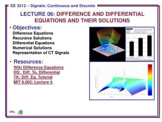
LECTURE 06: DIFFERENCE AND DIFFERENTIAL EQUATIONS AND THEIR SOLUTIONS. Objectives: Difference Equations Recursive Solutions Differential Equations Numerical Solutions Representation of CT SIgnals

E N D
LECTURE 06: DIFFERENCE AND DIFFERENTIAL EQUATIONS AND THEIR SOLUTIONS • Objectives:Difference EquationsRecursive SolutionsDifferential EquationsNumerical SolutionsRepresentation of CT SIgnals • Resources:Wiki Difference EquationsDS: Diff. To. DifferentialTK: Diff. Eq. TutorialMIT 6.003: Lecture 4 URL:
Linear Constant-Coefficient Difference Equations • We can model the input/output behavior of a DT LTI systems using an Nth-order input/output difference equation (also called a digital filter): DT LTI • Solution of such equations can be easily computed by solving for y[n]: • Let us consider a simple example: • Let us assume: (the latter are referred to as initial conditions). The output can be computed using a table:
Difference Equations in MATLAB • The solutions to these equations canbe easily programmed in MATLAB. • Note that the key step is actually a dot product between the equation’s coefficients and the previous samples of the output and input (often referred to as the filter memory). • The response to a unit step function can also be computed using the function recur. • The unit step function is created by assigning values of “1” to x, followed by the invocation of the recur function that performs the difference equation computations.
Complete Response of a First-Order Equation • Consider the first-order linear difference equation: • Let us assume that: • The first part of the response is due to the initial condition being nonzero. The second part of the response is due to the forcing function, x[n]. • Together, they comprise the complete response of the system. • We will see that closed-form solutions of these equations can be easily computed using the z-transform, which is very similar to the Laplace transform. The z-transform converts the difference equation to an algebraic equation. • Closed-form solutions can also be found using summation tables.
Differential Equations • For CT systems, such as circuits, our principal tool is the differential equation. • For the circuit shown, we can easily compute the input/output differential equation using Kirchoff’s Law. • What is the nature of the impulse response for this circuit?
Numerical Solutions to Differential Equations • Consider our 1st-order diff. eq.: • We can solve this numerically by setting t = nT: • The derivative can be approximated: • Substituting into our diff. eq.: • Let and : • We can replace n by n-1 to obtain: • This is called the Euler approximation to the differential equation. • With and initial condition, , the solution is: • The CT solution is: • Later, we will see that using the Laplace transform, we can obtain: • But we can approximate this: • Which tells us our 1st-order approximation is accurate!
Higher-Order Derivatives • We can use the same approach for the second-order derivative: • Higher-order derivatives can be similarly approximated. • Arbitrary differential equations can be converted to difference equations using this technique. • There are many ways to approximate derivatives and to numerically solve differential equations. MATLAB supports both symbolic and numerical solutions. • Derivatives are quite tricky to compute for discrete-time signals. However, in addition to the differences method shown above, there are powerful methods for approximating them using statistical regression. • Later in the course we will consider the implications of differentiation in the frequency domain.
Series RC Circuit Example Difference Equation: R=1;C=1;T=0.2; a=-(1-T/R/C);b=[0 T/R/C]; y0=0; x0=1; n=1:40; x=ones(1,length(n)); y1=recur(a, b, n, x, x0, y0); Analytic Solution: t=0:0.04:8; y2=1-exp(-t); y1=[y0 y1]; n=0:40; plot(n*T, y1, ’o’, t, y2, ’-’);
Representation of CT Signals • Recall from calculus how we approximated a function by a sum of time-shifted, scaled pulse functions: • We approximate the signal’s amplitude value as a constant over the interval : • The signal changes discontinuously at the next step. • What happens as ? Recall ourrepresentation of a CT impulse function:
Representation of CT Signals Using Impulse Functions • We approximate a CT signalas a weighted pulse function. • The signal can be written as a sum of these pulses: • In the limit, as : • Mathematical definition of an impulsefunction (the equivalent of the unit pulsefor DT signals and systems): • Unit pulses can be constructed from many functional shapes (e.g., triangular or Gaussian) as long as they have a vanishingly small width. The rectangular pulse is popular because it is easy to integrate
Summary • We introduced a linear constant coefficient difference equation. • We demonstrated how to solve such equations numerically. • We demonstrated how these difference equations can be used to approximate differential equations. • We discussed how to convert derivatives to differences. • We compared the accuracy of the analytic and approximate solutions for a series RC circuit. • We introduced a method for representing CT signals as a combination of impulse functions. We will use this representation to derive the convolution integral for CT signals.