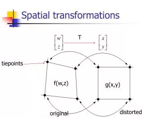
Spatial transformations

1. Spatial transformations T tiepoints f(w,z) g(x,y) distorted original

2. Affine transform MATLAB code: T=[2 0 0; 0 3 0; 0 0 1]; tform=maketform('affine', T); tform.tdata.T tform.tdata.Tinv WZ=[1 1; 3 2]; XY=tformfwd(WZ, tform); WZ2=tforminv(XY, tform);

3. Exercise#1 % generate a grid image [w, z]=meshgrid(linspace(0,100,10), linspace(0,100,10)); wz = [w(:) z(:)]; plot(w, z, 'b'), axis equal, axis ij hold on plot(w', z', 'b'); set(gca, 'XAxisLocation', 'top'); EX. Apply the following T to the grids, and plot all results T1 = [3 0 0; 0 2 0; 0 0 1]; T2 = [1 0 0; .2 1 0; 0 0 1]; T3 = [cos(pi/4) sin(pi/4) 0; -sin(pi/4) cos(pi/4) 0; 0 0 1];

4. Apply spatial transformations to images • Inverse mapping then interpolation distorted original

5. Apply spatial transformations to images (cont.) • MATLAB function • Ex#2 g=imtransform(f, tform, interp); f=checkerboard(50); Apply T3 to f with ‘nearest’, ‘bilinear’, and ‘bicubic’ interpolation method. Zoom the resultant images to show the differences.

6. Tiepoints after distortion original Nearest neighbor restored distorted Bilinear interp. restored distorted

7. original distorted (Using Previous Slide) restored Diff.

8. Image transformation using control points • Ex#3, for original f and transformed g in Ex#2, using cpselect tool to select control points: cpselect(g, f); With input_points and base_points generated using cpselect, we do the following to reconstruct the original checkerboard. tform=cp2tform(input_points, base_points, 'projective'); gp=imtransform(g, tform);

9. Project#3: iris transformation • Polar coordinate to Cartesian coordinate • Check the reference paper

10. Image Topology

11. Motivation • How many rice?

12. Outline • Neighbors and adjacency • Path, connected, and components • Component labeling • Lookup tables for neighborhood

13. Neighborhood and adjacency • 4-neighbors • 8-neighbors Q P P and Q are 4-adjacent Q P and Q are 8-adjacent P

14. Q P P and Q are 8-connected The above set of pixels are 8-connected. => 8-component Path, connected and components Q P P and Q are 4-connected The above set of pixels are 4-connected. => 4-component

15. Component labeling • Two 4-components. How to label them?

16. Component labeling algorithm • Scan left to right, top to down. • Start from top left foreground pixel. • 2. Check its upper and left neighbors. • Neighbor labeled => take the same label • Neighbor not labeled => new label 1 2 1 3 3 4 4 5

17. 1 1 2 1 1 1 3 2 2 3 4 2 4 2 2 5 Component labeling algorithm {1,2} and {3,4,5} are equivalent classes of labels, which are defined by adjacent relation. {1,2} => 1 {3,4,5} => 2

18. Ex#4: component labeling • MATLAB code • Threshold the rice.tiff image, then count the number of rice. Using 4- and 8-neighbors. Show the label image and the number of rice in the title. i=zeros(8,8); i(2:4,3:6)=1; i(5:7,2)=1; i(6:7,5:8)=1; i(8,4:5)=1; bwlabel(i,4) bwlabel(i,8)

19. Lookup tables for neighborhood • For a 3x3 neighborhood, there are 29=512 possible • For each possible neighborhood, give it a unique number(類似2進位編碼) 8 64 1 = 3 2 128 16 .X 4 32 256

20. Lookup tables for neighborhood (cont.) • Performing any possible 3x3 neighborhood operation is equivalent to table lookup Input Output 1 0 2 1 … … 2 511

21. Ex#5: table lookup • Find the boundary that are 4-connected in a binary image • Ex#5: Find the 8-boundary of the rice image using lookup table f=inline('x(5) & ~(x(2)*x(4)*x(6)*x(8))'); lut=makelut(f,3); Iw=applylut(II, lut);

22. Ex#6: table lookup • Build lookup tables for the following cases • Show your result with the following matrix a=zeros(8,8); a(2,2)=1; a(4:8,4:8)=1; a(6,6)=0;