Structure determination from X-ray powder diffraction data
Structure determination from X-ray powder diffraction data. Alok Kumar Mukherjee Department of Physics Jadavpur University Kolkata -700032 E-mail : akm_ju@rediffmail.com.

Structure determination from X-ray powder diffraction data
E N D
Presentation Transcript
Structure determination from X-ray powder diffraction data Alok Kumar Mukherjee Department of Physics Jadavpur University Kolkata -700032 E-mail : akm_ju@rediffmail.com
(i) Phase identification(ii) Quantitative phase analysis(iii) Microstructure study(iv) Texture analysis (v) Thin film study(vi) Dynamic and nonambient diffraction Crystal structure determination using X-ray powder diffraction is a far more difficult task than several other applications of X-ray powder diffraction, such as:
Single crystal versus powder crystal XRD Although the single crystal and powder crystal XRD patterns essentially contain the same information, but in the former case the information is distributed in three-dimensional space where as in the latter case the three-dimensional data are “compressed” into one-dimension. Single Crystal Diffraction Powder Diffraction
As a consequence, there is generally considerable overlap of peaks in the X-ray powder pattern leading to ambiguities in extracting the peak positions(2) and intensities, I(hkl), of individual diffraction maxima. The powder diffraction pattern
Why structure determination from powder XRD ? Many crystalline solids including several organic, metal-organic, pharmaceutical compounds and nano-materials are available only as polycrystalline powders. In such cases, X-ray powder diffraction is the only realistic option for structure elucidation.
Flow chart for structure determination from X-ray powder diffraction data High quality powder XRD data collection Measurement of step scanned intensity data Unit cell determination Indexing the XRD pattern Possible space group assignment Look for any obvious systematic absences Determination of approximate atomic positions Structure solution Refinement of atomic coordinates, temperature factors, occupancy factors Structure refinement
The whole procedure of structure determination from X-ray powder data is not automatic. It requires significant intelligent input from the crystallographer at every step during the process. For success in structure determination from powder diffractometry (SDPD), the first step i.e. data collection is crucial .
The quality of data sets necessary depends on the type of analysis intended. • Indexing requires accurate and precise peak positions, specially at low 2θ values (large d-spacings). • Structure solution requires reliable intensities. • Structure refinement requires good quality high angle data (small d-spacings).
In addition, high-resolution data (narrow 2θ peak width) is desirable. High sample purity is required. One potential adverse effect of using very high resolution powder diffractometers is that any impurity peaks from the sample are more easily seen → problem in indexing !
Some useful data collection parameters (i) Wave length of X-ray (usually CuK is used) (ii) Monochromatization (iii) Zero-shift alignment (iv) Incident and diffracted beam apertures Divergent slit ~ 0.1 mm – 0.6 mm Receiving slit ~ 0.1 mm – 0.2 mm (v) Data collection parameters (Step scan mode) (a) Step size ~ 0.008º - 0.02º (b) Counting time ~ 20 - 30 sec/step Data acquisition variables can be adjusted to produce a better quality data set.
Sample holder X-ray tube Detector Slit boxes The view of Bruker D8 Advance diffractometerwith stationary X-ray source and synchronized rotations of both the detector arm and sample holder
Some criteria for good quality X-ray powder data • Peak to noise ratio • should be high • Full width half maxima • peak overlapping (~ 0.08º- 0.10º) • 3. Number of peaks • 4. Reproducibility of powder pattern • preferred orientation
Number of expected diffraction peaks The number of reflections up to the diffraction angle θ in a powder diffraction pattern is determined by the size and symmetry of the unit cell and the wavelength of the radiation used. N=32πVSin2θ/3λ3Q , Where V is the unit cell volume, λ is the wavelength and Q is the product of the average multiplicity of the reflections and the number of lattice points per unit cell.
For example: λ= 1.5418Å, V= 1500 Å3 , 2θ= 25° N =32πVSin2θ/3λ3Q = 637/Q For orthorhombic system : Q = average multiplicity X no. of lattice points per unit cell = 5 X 1 = 5 and N = 637/5 ≈ 127
Effect of counting time on statistical error during a single measurement Counts Counting Number (N) of Spread (√N) Error ()at 90% Error ()at 99% per sec time (s) registered counts confidence(%) confidence(%) 100 1 100 10 16.4 25.9 100 25 2500 50 3.3 5.2 =[Q/(N)½] x 100%, Q=1.64 for 90% confidence level Q=2.59 for 99% confidence level
Particular problem with organic and pharmaceutical compounds ~ diffraction data often contain very few peaks
Effect of the divergence slit width Slit with 0.05mm Slit with 0.6mm
Effect of the divergence slit width in peak asymmetry Slit with 0.05mm Slit with 0.6mm
Powder pattern indexing The basic equation used for indexing a powder diffraction pattern is Qhkl = 1/dhkl2 = h2a*2+k2b*2+l2c*2+2klb*c*cos*+ 2hlc*a*cos*+2hka*b*cos* where, dhkl is the interplanar spacing corresponding to the (hkl) plane and a*, b*, c*, *, *, * are the reciprocal lattice cell parameters.
The 2θ positions corresponding to a reasonable number of diffraction maxima (say 20-30) are extracted from the observed pattern by fitting individual peaks using appropriate profile function. Different Indexing programs: TREOR → A semi-exhaustive trial-and-error indexing program, which is based on the permutation of Miller indices in a selected basis set of lowest Bragg angle peaks. DICVOL → An exhaustive trial-and-error indexing program based on the variation of the lengths of cell edges and inter-axial angles over finite ranges, followed by a progressive reduction of these intervals by means of a dichotomy procedure.
ITO → A zone search indexing method with the provision for the reduction of the most probable unit cell. It is based on specific relations among Qhkl values in reciprocal space. MCMAILLE → Based on the Monte Carlo and grid search method. X-cell→ An indexing algorithm which uses an extinction-specific dichotomy procedure to perform an exhaustive search of parameter space to establish a complete list of all possible unit cell solutions.
Commonly used figures of merit To assess the reliability of indexing, two figures of merit are commonly used. The de Wolff ’s figure of merit (M20) M20= Q20 / 2N20 x (ΔQ)av where, Q20 is the Q value (1/d2) for the 20th observed line, N20 is the number of different diffraction lines possible up to the 20th observed line, (ΔQ)av is the average absolute discrepancy between the observed and calculated Q values for the 20 observed lines.
The Smith and Snyder figure of merit (FN) FN= N / Npossx (Δ2)av Where Nposs is the number of calculated diffraction lines up to the Nth observed line and (Δ2)av is the average absolute discrepancy between the observed and calculated 2 values. Higher the accuracy of the data collected and more complete the pattern, the larger will be M20 and FN values.
Comments on the value of M20 • A ‘solution’ with FOM value less than 5.0 is worthless. • Any ‘solution’ that leaves more than two very weak lines unexplained is not useful. However, if the FOM is greater than 10.0 it might be worthwhile to examine the input data and the ‘solution’ more closely. • Even ‘solutions’ that index all lines with a FOM > 10.0 should not be accepted uncritically without further investigation. Experience shows that M20 values greater than 15 are likely to correspond to correct solutions for laboratory X-ray powder data.
Pitfalls in indexing: • Attempting to index a poor data is a non-starter → trying to solve a jigsaw puzzle with half the pieces missing !!
Pseudo-symmetry: when certain lattice parameters have values that result in the symmetry of the lattice appearing to be higher than reality e.g. , • → Monoclinic angle β very close to 90°, the metric tensor for the lattice will be similar to that of an orthorhombic lattice. • → unit cell has a monoclinic symmetry, but a≈c and γ close to 120°; the symmetry of the lattice is then pseudo-hexagonal. • Instrumental errors: • Satisfactory solution may not be obtained if 2θ zero error greater than 0.08° .
Dominant Zones Indexing a powder pattern with dominant zones (one cell axis is much shorter than the other two) is often a problem. If most of the first few lines are of h0l type → the d-spacings intrinsically lack 3-dimensional unit cell information. To overcome this problem XRD pattern should be collected of an unground powder sample.
Impurities and other phases: • Which peak(s) due to impurity ? • Samples that change phase during data acquisition
Indexing of the XRD data collected with step size 0.02º and counting time 20s per step results a triclinic cell with low FOM. Crystal system : Triclinic a=4.734(4) Å, α=92.1(1)º b=8.248(6) Å β=85.8(1)º c=10.811(7) Å γ=98.0(1)º Vol=416.7 Å3 F20= 23, M20= 15 No corresponding calculated position WPPD plot
Indexing of the same XRD data collected with step size 0.008º and counting time 30sper step results a orthorhombic cell with high FOM. Crystal system : Orthorhombic a=16.666(2) Å b=10.548(2) Å c=9.476(2) Å Vol=1665.8 Å3 F20= 88, M20= 52 WPPD plot
Space group assignment- most tricky part! The choice of space group is possibly the difficult part to automate. The presence or absence of screw axes or glide planes from indexing is not always obvious since the average powder pattern is likely to contain only a few reflections of the type h00 (or 0k0, 00l) and hk0 (or h0l , 0kl etc.). The paucity of data results in real ambiguities in the choice of space groups.
If there is a choice between a commonly observed space group and a rare one based on occurrence in the Cambridge Crystallographic Database (e.g P2/c vs P21/c), then try to solve the structure using the most common space group first.
Example: A molecular structure indexed in the orthorhombic system showed Z=8. The reflection conditions are ambiguous and indicate either Pbca or Pnma (this situation can easily arise due to overlap of key reflections in the powder pattern). Both these space groups are found to occur frequently for molecular compounds.
For Pnma, however, the presence of mirror plane would suggest either two molecules related by mirror symmetry or two molecules per asymmetric unit with the mirror plane passing through both molecules → unlikely situation from packing consideration. So, in this case the first choice should be Pbca
A better way to overcome this problem is to employ Whole pattern fitting approach in which the diffraction profile is fitted in the absence of a structural model, but in the presence of the reflection conditions of the various space groups under consideration. In EXPO-2004, for each crystal system, the probabilities of different extinction symbols are calculated. A list of possible space groups compatible with each extinction symbol is presented.
Successful structure solution will only ascertain the correctness of the assigned space group! Structure was solved in P21/a - which had a lower FOM
Structure solution Traditional methods (Patterson, Direct methods) Using the extracted intensities, the structure solution procedures are similar to those in the single crystal case. Direct space approach (Monte Carlo, Simulated annealing, Grid search etc.) All direct space approaches avoid the problematic step of Ihkl extraction from the experimental powder pattern Trial structural models generated in direct space. Suitability of a model assessed by comparing the calculated powder pattern based on the model with the observed powder pattern.
Monte Carlo approach In the Monte Carlo approach a sequence of structures is generated as potential structure solution. The first structure (x1) is generally chosen as a random position of the structural fragment in the unit cell. Starting from the structure xi, the structural fragment is subjected to a random displacement to generate a trial structure (xtrial). The trial structure is then accepted or rejected by considering the difference z between the Rwp values corresponding to structures xtrial and xi.
z = Rwp (xtrial) – Rwp (xi) if z ≤ 0, the trial structure is automatically accepted, whereas if z > 0, the trial structure is accepted with probability exp(-z/s) and rejected with probability [1-exp(-z/s)], where s is a scaling factor. After a sufficiently extensive range of structural space has been explored, the structure corresponding to lowest Rwp is considered as the starting model for refinement
The main factor limiting the efficiency of Monte Carlo calculation is the number of structural degrees of freedom varied during calculation. Thus in the Monte Carlo approach, the number of degrees of freedom in the structural fragment is a more important consideration than the number of atoms in the asymmetric unit. This approach is quite popular with organic or pharmaceutical compounds where the molecular compositions are known a priori.
Rietveld method In the Rietveld method, the integrated intensities of the reflections (Ihkl) are calculated from the atomic parameters of the model. The equations for y(2i)cal now becomes y(2i)cal = smhkl (Lp)hkl |Fhkl|2 Phkl hkl + b(2i) Where, s is the scale factor, mhkl is the reflection multiplicity, (Lp)hkl is the Lorentz-polarization factor, P is the preferred orientation function, is the reflection profile function, Fhkl is the structure factor for the reflection, b(2i) is the background intensity at the ith step.
Criteria of fit The agreement between the observed and calculated powder patterns is judged by several indicators. The profile R-factors are, R- pattern (profile) RP = |yi (obs) - yi (calc)| / |yi (obs)| R weighted pattern (profile) RwP= [ wi {yi (obs) - yi (calc)}2 / wi { yi (obs)}2]1/2 R-Structure factor RF= |(IK(obs))1/2 - (IK(calc))1/2| / (IK(obs))1/2
R-Bragg factor RB = |IK(obs) - IK(calc)| / |IK(obs)| R expected RE = [(N- P)/ wi { yi (obs)}2]1/2 Where, N and P are the number of profile points and refined parameters, respectively Goodness-of-fit 2 = (Rwp / RE)2
Example-1: 5-5′- disubstituted hydantoins Imidazolidine-2,4-dione, or hydantoin, is a five-membered heterocyclic ring containing a reactive cyclic urea nucleus. Hydantoins can serve as useful intermediates in the synthesis of amino acids.
Dipropyl glycine hydantoin The indexing with TREOR showed an orthorhombic unit cell with a= 7.167(1), b= 13.964(1), c =10.957(3)Å [M(20)= 49, F(20)= 84(0.003343, 72)] Statistical analysis of the using the FINDSPACE module of EXPO2004 indicated Pnma as the most probable space group (Z’= 0.5)