Introduction to SVMs

1. Introduction to SVMs

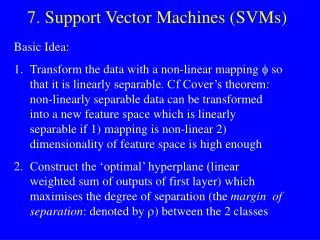
2. SVMs • Geometric • Maximizing Margin • Kernel Methods • Making nonlinear decision boundaries linear • Efficiently! • Capacity • Structural Risk Minimization

3. a Linear Classifiers x f yest f(x,w,b) = sign(w. x- b) denotes +1 denotes -1 How would you classify this data?

4. a Linear Classifiers x f yest f(x,w,b) = sign(w. x- b) denotes +1 denotes -1 How would you classify this data?

5. a Linear Classifiers x f yest f(x,w,b) = sign(w. x- b) denotes +1 denotes -1 How would you classify this data?

6. a Linear Classifiers x f yest f(x,w,b) = sign(w. x- b) denotes +1 denotes -1 Any of these would be fine.. ..but which is best?

7. a Classifier Margin x f yest f(x,w,b) = sign(w. x- b) denotes +1 denotes -1 Define the margin of a linear classifier as the width that the boundary could be increased by before hitting a datapoint.

8. a Maximum Margin x f yest f(x,w,b) = sign(w. x- b) denotes +1 denotes -1 The maximum margin linear classifier is the linear classifier with the maximum margin. This is the simplest kind of SVM (Called an LSVM) Linear SVM

9. a Maximum Margin x f yest f(x,w,b) = sign(w. x- b) denotes +1 denotes -1 The maximum margin linear classifier is the linear classifier with the, um, maximum margin. This is the simplest kind of SVM (Called an LSVM) Support Vectors are those datapoints that the margin pushes up against Linear SVM

10. Why Maximum Margin? • Intuitively this feels safest. • If we’ve made a small error in the location of the boundary (it’s been jolted in its perpendicular direction) this gives us least chance of causing a misclassification. • There’s some theory (using VC dimension) that is related to (but not the same as) the proposition that this is a good thing. • Empirically it works very very well. f(x,w,b) = sign(w. x- b) denotes +1 denotes -1 The maximum margin linear classifier is the linear classifier with the, um, maximum margin. This is the simplest kind of SVM (Called an LSVM) Support Vectors are those datapoints that the margin pushes up against

11. A “Good” Separator O O X X O X X O O X O X O X O X

12. Noise in the Observations O O X X O X X O O X O X O X O X

13. Ruling Out Some Separators O O X X O X X O O X O X O X O X

14. Lots of Noise O O X X O X X O O X O X O X O X

15. Maximizing the Margin O O X X O X X O O X O X O X O X

16. Specifying a line and margin • How do we represent this mathematically? • …in m input dimensions? Plus-Plane “Predict Class = +1” zone Classifier Boundary Minus-Plane “Predict Class = -1” zone

17. Specifying a line and margin Plus-Plane “Predict Class = +1” zone Classifier Boundary • Plus-plane = { x : w . x + b = +1 } • Minus-plane = { x : w . x + b = -1 } Minus-Plane “Predict Class = -1” zone wx+b=1 wx+b=0 wx+b=-1

18. Computing the margin width M = Margin Width “Predict Class = +1” zone • Plus-plane = { x : w . x + b = +1 } • Minus-plane = { x : w . x + b = -1 } Claim: The vector w is perpendicular to the Plus Plane. Why? How do we compute M in terms of w and b? “Predict Class = -1” zone wx+b=1 wx+b=0 wx+b=-1

19. Computing the margin width M = Margin Width “Predict Class = +1” zone • Plus-plane = { x : w . x + b = +1 } • Minus-plane = { x : w . x + b = -1 } Claim: The vector w is perpendicular to the Plus Plane. Why? How do we compute M in terms of w and b? “Predict Class = -1” zone wx+b=1 wx+b=0 wx+b=-1 Let u and v be two vectors on the Plus Plane. What is w . ( u – v ) ? And so of course the vector w is also perpendicular to the Minus Plane

20. Computing the margin width M = Margin Width x+ “Predict Class = +1” zone • Plus-plane = { x : w . x + b = +1 } • Minus-plane = { x : w . x + b = -1 } • The vector wis perpendicular to the Plus Plane • Let x- be any point on the minus plane • Let x+ be the closest plus-plane-point to x-. • Claim: x+ = x- + lw for some value of l. Why? How do we compute M in terms of w and b? x- “Predict Class = -1” zone wx+b=1 wx+b=0 wx+b=-1

21. Computing the margin width M = Margin Width x+ “Predict Class = +1” zone What we know: • w . x+ + b = +1 • w . x- + b = -1 • x+ = x- + lw • |x+ - x- | = M It’s now easy to get M in terms of w and b x- “Predict Class = -1” zone wx+b=1 wx+b=0 wx+b=-1

22. Computing the margin width M = Margin Width x+ “Predict Class = +1” zone What we know: • w . x+ + b = +1 • w . x- + b = -1 • x+ = x- + lw • |x+ - x- | = M It’s now easy to get M in terms of w and b x- “Predict Class = -1” zone wx+b=1 w . (x - + lw) + b = 1 => w . x -+ b + lw .w = 1 => -1 + lw .w = 1 => wx+b=0 wx+b=-1

23. Computing the margin width M = Margin Width = x+ “Predict Class = +1” zone What we know: • w . x+ + b = +1 • w . x- + b = -1 • x+ = x- + lw • |x+ - x- | = M x- “Predict Class = -1” zone wx+b=1 M = |x+ - x- | =| lw |= wx+b=0 wx+b=-1

24. Learning the Maximum Margin Classifier M = Margin Width = x+ “Predict Class = +1” zone Given a guess of w and b we can • Compute whether all data points in the correct half-planes • Compute the width of the margin So now we just need to write a program to search the space of w’s and b’s to find the widest margin that matches all the datapoints. How? Gradient descent? Simulated Annealing? Matrix Inversion? EM? Newton’s Method? x- “Predict Class = -1” zone wx+b=1 wx+b=0 wx+b=-1

25. Don’t worry… it’s good for you… • Linear Programming find w argmax cw subject to wai  bi, for i = 1, …, m wj  0, for j = 1, …, n There are fast algorithms for solving linear programs including the simplex algorithm and Karmarkar’s algorithm

26. Quadratic Programming Quadratic criterion Find Subject to n additional linear inequality constraints And subject to e additional linear equality constraints

27. Quadratic Programming Quadratic criterion Find There exist algorithms for finding such constrained quadratic optima much more efficiently and reliably than gradient ascent. (But they are very fiddly…you probably don’t want to write one yourself) Subject to n additional linear inequality constraints And subject to e additional linear equality constraints

28. Learning the Maximum Margin Classifier M = “Predict Class = +1” zone Given guess of w , b we can • Compute whether all data points are in the correct half-planes • Compute the margin width Assume R datapoints, each (xk,yk) where yk = +/- 1 “Predict Class = -1” zone wx+b=1 wx+b=0 wx+b=-1 What should our quadratic optimization criterion be? How many constraints will we have? What should they be? R Minimizew.w w . xk + b >= 1 if yk = 1 w . xk + b <= -1 if yk = -1

29. Large-margin Decision Boundary • The decision boundary should be as far away from the data of both classes as possible • We should maximize the margin, m • Distance between the origin and the linewtx=k is k/||w|| Class 2 m Class 1

30. Finding the Decision Boundary • Let {x1, ..., xn} be our data set and let yiÎ {1,-1} be the class label of xi • The decision boundary should classify all points correctly Þ • The decision boundary can be found by solving the following constrained optimization problem • This is a constrained optimization problem. Solving it requires some new tools • Feel free to ignore the following several slides; what is important is the constrained optimization problem above

31. Back to the Original Problem • The Lagrangian is • Note that ||w||2 = wTw • Setting the gradient of w.r.t. w and b to zero, we have

32. The Karush-Kuhn-Tucker conditions, • If , then , or in other word, is on the boundary of the slab; • If , is not on the boundary of the slab, and .

33. The Dual Problem • If we substitute to , we have • This is a function of ai only

34. The Dual Problem • It is known as the dual problem: if we know w, we know all ai; if we know all ai, we know w • The objective function of the dual problem needs to be maximized! • The dual problem is therefore: Properties of ai when we introduce the Lagrange multipliers The result when we differentiate the original Lagrangian w.r.t. b

35. The Dual Problem • This is a quadratic programming (QP) problem • A global maximum of ai can always be found • w can be recovered by

36. Characteristics of the Solution • Many of the ai are zero • w is a linear combination of a small number of data points • xi with non-zero aiare called support vectors (SV) • Let tj (j=1, ..., s) be the indices of the s support vectors. We can write • For testing with a new data z • classify z as class 1 if the sum is positive, and class 2 otherwise

37. A Geometrical Interpretation Class 2 a10=0 a8=0.6 a7=0 a2=0 a5=0 a1=0.8 a4=0 a6=1.4 a9=0 a3=0 Class 1

38. Class 2 Class 1 Non-linearly Separable Problems • We allow “error” xi in classification; it is based on the output of the discriminant function wTx+b • xi approximates the number of misclassified samples

39. Learning Maximum Margin with Noise M = e11 e2 wx+b=1 e7 wx+b=0 wx+b=-1 The quadratic optimization criterion: Minimize How many constraints will we have? R Constraint:

40. Learning Maximum Margin with Noise m = # input dimensions Our original (noiseless data) QP had m+1 variables: w1, w2, … wm, and b. Our new (noisy data) QP has m+1+R variables: w1, w2, … wm, b, ek , e1 ,… eR R= # samples The quadratic optimization criterion: Minimize How many constraints will we have? 2R Constraint:

41. An Equivalent Dual QP Minimize The Lagrange function:

42. An Equivalent Dual QP The Lagrange function: • Setting the respective derivatives to zero, we get

43. An Equivalent Dual QP Minimize Dual QP Maximize where Subject to these constraints:

44. Then define: An Equivalent Dual QP Maximize where Subject to these constraints: Then classify with: f(x,w,b) = sign(w. x- b)

45. Nonlinear Classification Problem

46. Example XOR problem revisited: Let the nonlinear mapping be : f(x)=(1,x12, 21/2 x1x2, x22, 21/2 x1 , 21/2 x2)T And: f(xi)=(1,xi12, 21/2 xi1xi2, xi22, 21/2 xi1 , 21/2 xi2)T Therefore the feature space is in6Dwith input data in 2D x1 = (-1,-1), d1= - 1 x2 = (-1, 1), d2= 1 x3 = ( 1,-1), d3= 1 x4 = (-1,-1), d4= -1

47. Q(a)= S ai – ½ S S ai aj di dj f(xi) Tf(xj) =a1 +a2 +a3 +a4 – ½(9 a1 a1 - 2a1 a2 -2 a1 a3 +2a1 a4 +9a2 a2 + 2a2 a3 -2a2 a4 +9a3 a3 -2a3 a4 +9 a4 a4 ) To minimize Q, we only need to calculate (due to optimality conditions) which gives 1=9 a1 - a2 -a3 +a4 1= -a1 + 9 a2 +a3 -a4 1= -a1 + a2 +9 a3 -a4 1=a1 - a2 - a3 + 9a4

48. The solution of which gives the optimal values: a0,1 =a0,2 =a0,3 =a0,4 =1/8 w0 = S a0,i di f(xi) = 1/8[f(x1)- f(x2)- f(x3)+ f(x4)] Where the first element of w0 gives the bias b

49. From earlier we have that the optimal hyperplane is defined by: w0Tf(x) = 0 That is: w0Tf(x) which is the optimal decision boundary for the XOR problem. Furthermore we note that the solution is unique since the optimal decision boundary is unique

50. Output for polynomial RBF