Download
1 / 33
330 likes | 355 Views
Support Vector Machines Most of the slides were taken from: http://www.csd.uwo.ca/~olga/Courses/CS434a_541a/Lecture11.pdf. Support Vector Machines (SVMs). Originated in 1979 by a paper By Vladimir Vapnik The major development were invented mostly in the 1990’s

E N D
Support Vector MachinesMost of the slides were taken from:http://www.csd.uwo.ca/~olga/Courses/CS434a_541a/Lecture11.pdf
Support Vector Machines (SVMs) • Originated in 1979 by a paper By Vladimir Vapnik • The major development were invented mostly in the 1990’s • Its roots are in linear classification • But it has non-linear extensions • It has a very elegant (though very difficult) mathematical background • The learning problem will be solved by quadratic optimization, which will lead to a globally optimal solution • It has been successfully applied to a lot of machine learning problems in the last 20 years • It was the most successful and most popular machine learning algorithm in the 90’s
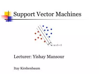
Let’s return to linear discriminant functions • In the linearly separable case usually there are a lot of possible solutions • Which one should we prefer from among the red lines?
Linear discriminant functions • Remember that the training data items are just samples from all the possible data • Our goal is to generalize tounseen data • A new sample from a class is likely to be close to the trainingsamples from the same class • So if the decision boundary is close to the training samples, then the new sample will fall onthe wrong side misclassification • Our heuristic here will be that putting the decision boundary as far from the samples as possible will hopefully increase generalization
Support Vector Machines – Basic Idea • Our basic ideas will be to move the hyperplane as fas as possible from the training data • For the optimal hyperplane the distance from the nearest example from class 1 will be the same as the distance from the nearest example from class 2
SVMs – Linearly Separable Case • SVMs will seek to maximize the margin • Where the margin is twice the distance of the closest example to the separating hyperplane • Maximizing the margin leads to a better generalization • Both is theory and in practice
SVMs – Linearly Separable Case • The support vectors are the samples that are the closest to the separa-ting hyperplane • These samples are the most difficult to classify • The separating hyperplane is completely defined by the support vectors • But of course, we will know which samples are the support vectors only after finding the optimal hyperplane
Formalizing the margin • Remember that the distance of any x point from the separating hyperplane where g(x)=0 can be calculated as • And the distance remains the same if we multiply g(x) by a non-zero constant: • This means that minimizing the margin does not uniquely define g(x) • To make the largest margin hyperplane unique, we also require for any support vector xi
Formalizing the margin • With this restriction for all the support vectors • And the size of the margin is:
Maximizing the margin • We want to maximize the margin • So that all the samples are correctly classifiedand fall outside the margin: • Similar to the normalization step for linear classifiers, we want multiply the inequalitiesfor the negative class by -1 • For this, we introduce the variable z:
Maximizing the margin • We will maximize the margin by minimizing its reciprocal • with the constraint: • J(w) is a quadratic function, so it has a single global minimum • The optimization should be solved with satisfying linear constraints • This altogether leads to a quadratic programming task • According to the Kuhn-Tucker theorem, the problem is equivalent to • Where αi are new variables (one for each example)
Maximizing the margin • LD(α) can also be written as • Where H is an nxn matrix with • LD(α) can be optimized by quadratic programming • Let’s suppose we found the optimal α=(α1,…, αn) • Then for each training sample either αi=0or αi≠0 and • The samples for which αi≠0 will be the support vectors!
Maximizing the margin • We can calculate w as • And we can obtain w0 by taking any support vector xi for which αi>0: • The final discriminant function will be given as Where S is the set of support vectors • Notice that the discriminant function depends only on the support vectors, and it is independent of all the other training samples! • Unfortunately, the number of support vectors usually increases linearly with the number of training samples • Training SVMs is slow: requires operations with the nxn matrix H • A lot of efforts have been made to reduce the training time of SVMs
SVMs – linearly non-separable case • Most real-life tasks are linearly non-separable – can we still apply SVMs in this case? • Yes, but will have to allow samples to fall on the wrong side • And punish these samples during optimization • For this we introduce the variables ξ1,…, ξn(one for each training sample) • ξ1 depends on the distance of xi from the margin • We use ξ=0 for samples that on the right side, and also outside the margin • 0<ξ1<1 means mean that the sample is on the right side, but within the margin • ξ>1 means that the sample is on the wrong side • We change the constraints from to(“soft margin”)
SVMs – linearly non-separable case • We extend the target function to be minimized as • Where C is a parameter which allows to tune the importance of the newly introduced “punishment term” • Larger C allows fewer samples to be in a suboptimal position • Smaller C allows more samples to be in a suboptimal position
SVMs – linearly non-separable case • So we have to minimize • With the constraints • The Kuhn-Tucker theorem turns this into the quadratic programming problem • And the solution can be obtained very similarly to the separable case • Only the constraints have been modified
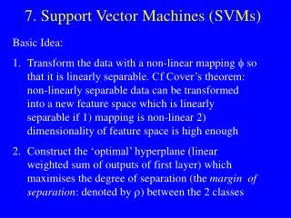
Non-linear SVMs • The linear SVM still uses a linear discriminant function • It is not flexible enough to solve real-life problems • We will create a non-linear extension of the SVM method by (non-linearly) projecting the training data into a larger dimensional space • Cover’s theorem: a pattern-classification problem cast in a high dimensional space non-linearly is more likely to be linearly separable than in a low-dimensional space • Example: 1D task, linearly non-separable 2D task, linearly separable • Where the features for newly introduced dimension are obtained as x2
Non-linear SVMs • We will denote the function that project the data into the new feature space by φ(x) • The steps of non-linear classification will be: • Project the data points into the new feature space using φ(x) • Find the linear discriminant function in this new feature space • Project the discriminant function back to the original space, where it won’t be linear:
Yet another example • The data is not linearly separable in the original 2D space, but it becomes linearly separable in the projected 3D space
Classifying in higher dimension • Projecting the data into a higher dimensional space makes the classes linearly separable • But what are the risks of working in a higher dimensional space? • The risk of overfitting increases (remember the “curse of dimensionality”!) • The computational complexity increases • Fortunately, the SVM training algorithm is quite insensitive to the number of dimensions • It can be shown that the generalization capability of an SVM depends on the margin found, and not on the number of dimensions • Computation in the higher dimensional space can be performed implicitly by the use of kernel functions • This will allow us even to work in an infinite-dimensional space!
The “kernel trick” • Remember that our function to be maximized was formulated as • It does not require the training vectors directly, only their pairwise inner products xitxj • If we project the samples into a higher dimensional space by using φ(x) instead of x, then The above formula will require φ(xit)φ(xj) • We would like to avoid the computation of these inner products directly, as these vector have a high dimension • The solution (“Kernel trick”): we find a kernel function K(xi,xj) for which • This way, instead of calculating φ(xit) and φ(xj) and then taking their inner product, we will have to calculate only K(xi,xj), which is in the original lower-dimensional space!
Kernel functions • Of course, not all possible K(xi,xj) functions will correspond to an inner product φ(xit)φ(xj) in a higher dimensional space • So we cannot just randomly select any K(xi,xj) function • The Mercer condition tells us which K(xi,xj) function in the original space can be expressed as a dot product in another space • Example: Suppose we have only two features • And the kernel function will be • We show that it can be written as an inner product: • We managed to write K(x, y) as an inner product with
Kernel functions in practice • As kernel functions are hard to find, in practice we usually apply some standard, well-known kernel functions • The popular kernel functions: • Polinomial kernel: • Gaussian or radial basis function (RBF) kernel (corresponds to a projection into infinite-dimensional space!): • For a huge list of possible kernel functions, see: • http://crsouza.com/2010/03/17/kernel-functions-for-machine-learning-applications/ • Unfortunately, in practice it is very difficult to tell which kernel function will work well for a given machine learning task
The discriminant function • SVM finds a linear discriminant function in the high-dimensional space: • How will it look like in the original space? • Let’s examine only the case when the first component of φ(x) is 1, eg: • In this case wφ(x) will already contain a component which is independent of x. As it will play the role of w0, we can restrict ourselves to discriminant functions that have the form
The discriminant function • Remember that the linear SVM maximizes • If we project our data into a higher dimensional space using φ(x), than the problem turns into • For the linear case we obtained the weight vector as • Now it becomes
The discriminant function • The discriminant function in the high dimensional space is linear • The discriminant function in the original space is: • Which will be non-linear is the kernel function is non-linear
Example – The XOR problem • The classification task is to separate two classes with 2-2 samples: • Class 1: x1=[1,-1] x2=[-1,1] • Class 2: x3=[1,1] x4=[-1,-1] • This is the simplest task in 2D which is linearly non-separable • We will apply the kernel function • Which corresponds to the mapping • And we have to maximize • With the constraints
Example – The XOR problem • The solution is α1= α2= α3= α4=0.25 • Which also means that all the 4 samples are support vectors • Remember that the transformed feature space has 6 dimensions calculated as • So the weight vector of the linear discriminant in this space has 6 components: • Which has only 1 non-zero component • The discriminant function in the original feature space is:
Example – The XOR problem • The decision boundary where g(x)=0 • It is non-linear in the original 2Dfeature space, while it is linear in the new 6D feature space (from which only 2 dimensions are shown in the figure), and it also correctly separates the two classes
Example – RBF kernel • The kernel function is • You can see how the decision boundaries change with the meta-parameters C (it is the parameter of SVM) and gamma (it is the parameter of the kernel function)
SVM extensions • Multi-class classification: • It is not easy to extend SVMs to multi-class classification • As the simplest solution, one can use the “one against the rest” or the “one against one” method presented earlier • Probability estimation • The SVM outputs cannot be directly interpreted as posterior probability estimates. There exists several solutions to convert their outputs to probability estimates, but these are just approximations • Regression • SVMs have several extensions which allow them to solve regression tasks instead of classification
SVM - Summary • Advantages: • It is based on a nice theory • It has good generalization properties (not inclined to overfitting) • It is guaranteed to find the global optimum • With the “kernel trick” it is able to find non-linear discriminant functions • The complexity of the learned classifier depends on the number of support vectors found, not on the number of training samples, nor on the number of dimensions of the transformed space • Disadvantages • The quadratic programming optimization is computationally more expensive than most of the other machine learning methods • Chosing the optimal kernel function is difficult