Descriptive Data Summarization (Understanding Data)
Descriptive Data Summarization (Understanding Data). Remember: 3VL. NULL corresponds to UNK for unknown u or unk also represended by NULL

Descriptive Data Summarization (Understanding Data)
E N D
Presentation Transcript
Remember: 3VL • NULL corresponds to UNK for unknown • u or unk also represended by NULL • The NULL value can be surprising until you get used to it. Conceptually, NULL means a missing unknown valueモ and it is treated somewhat differently from other values. To test for NULL, you cannot use the arithmetic comparison operators such as =, <, or <>. • 3VL a mistake?
Visualizing one Variable • Statistics for one Variable • Joint Distributions • Hypothesis testing • Confidence Intervals
Visualizing one Variable • A good place to start • Distribution of individual variables • A common visualization is the frequency histogram • It plots the relative frequencies of values in the distribution
To construct a histogram • Divide the range between the highest and lowest values in a distribution into several bins of equal size • Toss each value in the appropriate bin of equal size • The height of a rectangle in a frequency histogram represents the number of values in the corresponding bin
The choice of bin size affects the details we see in the frequency histogram • Changing the bin size to a lower number illuminates things that were previously not seen
Bin size affects not only the detail one sees in the histogram but also one‘s perception of the shape of distribution
Statistics for one Variable • Sample Size • The sample size denoted by N, is the number of data items in a sample • Mean • The arithmetic mean is the average value, the sum of all values in the sample divided by the number of values
Statistics for one Variable • Median • If the values in the sample are sorted into a nondecreasing order, the median is the value that splits the distribution in half • (1 1 1 2 3 4 5) the median is 2 • If N is even, the sample has middle values, and the median can be found by interpolating between them or by selecting one of the arbitrary
Mode • The mode is the most common value in the distribution • (1 2 2 3 4 4 4) the mode is 4 • If the data are real numbers mode nearly no information • Low probability that two or more data will have exactly the same value • Solution: map into discrete numbers, by rounding or sorting into bins for frequency histograms • We often speak of a distribution having two or more modes • Distributions has two or more values that are common
The mean, median and mode are measures of location or central tendency in distribution • They tell us where the distribution is more dense • In a perfectly symmetric, unimodal distribution (one peak), the mean, median and mode are identical • Most real distributions - collecting data - are neither symmetric nor unimodal, but rather, are skewed and bumpy
Skew • In a skewed distribution the bulk of the data are at one end of the distribution • If the bulk of the distribution is on the right, so the tail is on the left, then the distribution is called left skewed or negatively skewed • If the bulk of the distribution is on the left, so the tail is on the right, then the distribution is called right skewed or positively skewed • The median is to be robust, because its value is not distorted by outliers • Outliers: values that are very large or small and very uncommon
Symmetric vs. Skewed Data • Median, mean and mode of symmetric, positively and negatively skewed data
Trimmed mean • Another robust alternative to the mean is the trimmed mean • Lop off a fraction of the upper and lower ends of the distribution, and take the mean of the rest • 0,0,1,2,5,8,12,17,18,18,19,19,20,26,86,116 • Lop off two smallest and two larges values and take the mean of the rest • Trimmed mean is 13.75 • The arithmetic mean 22.75
Maximum, Minimum, Range • Range is the difference between maximun and minimum
Interquartile Range • Interquartile range is found by dividing a sorted distribution into four containing parts, each containing the same number • Each part is called quartile • The difference between the highest value in the third quartile and the lowest value in the second quartile is the interquartile range
Quartile example • 1,1,2,3,3,5,5,5,5,6,6,100 • The quartiles are • (1 1 2),(3 3 5),(5 5 5), (6,6,100) • Interquartile range 5-3=2 • Range 100-1=99 • Interquartile range is robust against outliers
Standard Deviation and Variance • Square root of the variance, which is the sum of squared distances between each value and the mean divided by population size (finite population) • Example • 1,2,15 Mean=6 • =6.37
Sample Standard Deviation and Sample Variance • Square root of the variance, which is the sum of squared distances between each value and the mean divided by sampe size (underlying larger population the sample was drawn) • Example • 1,2,15 Mean=6 • s=7.81
Because they are averages, both the mean and the variance are sensitive to outliers • Big effects that can wreck our interpretation of data • For example: • Presence of a single outlier in a distribution over 200 values can render some statistical comparisons insignificant
The Problem of Outliers • One cannot do much about outliers expect find them, and sometimes, remove them • Removing requires judgment and depend on one‘s purpose
Joint Distributions • Good idea, to see if some variable influence others
Scatter plot • Provides a first look at bivariate data to see clusters of points, outliers, etc • Each pair of values is treated as a pair of coordinates and plotted as points in the plane
Correlation Analysis • Correlation coefficient (also called Pearson’s product moment coefficient) where n is the number of tuples, and are the respective means of X and Y, σand σare the respective standard deviation of A and B, and Σ(XY) is the sum of the XY cross-product. • If rX,Y > 0, X and Y are positively correlated (X’s values increase as Y’s). The higher, the stronger correlation. • rX,Y = 0: independent; rX,Y < 0: negatively correlated
A is positive correlated • B is negative correlated • C is independent (or nonlinear)
Correlation Analysis • Χ2 (chi-square) test • The larger the Χ2 value, the more likely the variables are related • The cells that contribute the most to the Χ2 value are those whose actual count is very different from the expected count • Correlation does not imply causality • # of hospitals and # of car-theft in a city are correlated • Both are causally linked to the third variable: population
Chi-Square Calculation: An Example • Χ2 (chi-square) calculation (numbers in parenthesis are expected counts calculated based on the data distribution in the two categories) • It shows that like_science_fiction and play_chess are correlated in the group
Properties of Normal Distribution Curve • The normal (distribution) curve • From μ–σ to μ+σ: contains about 68% of the measurements (μ: mean, σ: standard deviation) • From μ–2σ to μ+2σ: contains about 95% of it • From μ–3σ to μ+3σ: contains about 99.7% of it
Kinds of data analysis • Exploratory (EDA) – looking for patterns in data • Statistical inferences from sample data • Testing hypotheses • Estimating parameters • Building mathematical models of datasets • Machine learning, data mining… • We will introduce hypothesis testing
The logic of hypothesis testing • Example: toss a coin ten times, observe eight heads. Is the coin fair (i.e., what is it’s long run behavior?) and what is your residual uncertainty? • You say, “If the coin were fair, then eight or more heads is pretty unlikely, so I think the coin isn’t fair.” • Like proof by contradiction: Assert the opposite (the coin is fair) show that the sample result (≥ 8 heads) has low probability p, reject the assertion, with residual uncertainty related to p. • Estimate p with a sampling distribution.
Probability of a sample result under a null hypothesis • If the coin were fair (p= .5, the null hypothesis) what is the probability distribution of r, the number of heads, obtained in N tosses of a fair coin? Get it analytically or estimate it by simulation (on a computer): • Loop K times • r := 0 ;; r is num.heads in N tosses • Loop N times ;; simulate the tosses • Generate a random 0 ≤ x ≤ 1.0 • If x < p increment r ;; p is the probability of a head • Push r onto sampling_distribution • Print sampling_distribution
Frequency (K = 1000) Probability of r = 8 or more heads in N = 10 tosses of a fair coin is 54 / 1000 = .054 70 60 50 40 30 20 10 0 1 2 3 4 5 6 7 8 9 10 Number of heads in 10 tosses Sampling distributions This is the estimated sampling distribution of r under the null hypothesis that p = .5. The estimation is constructed by Monte Carlo sampling.
0 1 2 3 4 5 6 7 8 9 10 The logic of hypothesis testing • Establish a null hypothesis: H0: p = .5, the coin is fair • Establish a statistic: r, the number of heads in N tosses • Figure out the sampling distribution of r given H0 • The sampling distribution will tell you the probability p of a result at least as extreme as your sample result, r = 8 • If this probability is very low, reject H0 the null hypothesis • Residual uncertainty is p
A common statistical test: The Z test for different means • A sample N = 25 computer science students has mean IQ m=135. Are they “smarter than average”? • Population mean is 100 with standard deviation 15 • The null hypothesis, H0, is that the CS students are “average”, i.e., the mean IQ of the population of CS students is 100. • What is the probability p of drawing the sample if H0 were true? If p small, then H0 probably false. • Find the sampling distribution of the mean of a sample of size 25, from population with mean 100
Central Limit Theorem: The sampling distribution of the mean is given bythe Central Limit Theorem The sampling distribution of the mean of samples of size N approaches a normal (Gaussian) distribution as N approaches infinity. If the samples are drawn from a population with mean and standard deviation , then the mean of the sampling distribution is and its standard deviation is as N increases. These statements hold irrespective of the shape of the original distribution.
100 135 The sampling distribution for the CS student example • If sample of N = 25 students were drawn from a population with mean 100 and standard deviation 15 (the null hypothesis) then the sampling distribution of the mean would asymptotically be normal with mean 100 and standard deviation The mean of the CS students falls nearly 12 standard deviations away from the mean of the sampling distribution Only ~1% of a normal distribution falls more than two standard deviations away from the mean The probability that the students are “average” is roughly zero
The Z test Mean of sampling distribution Sample statistic Mean of sampling distribution Test statistic std=3 std=1.0 100 135 0 11.67
Reject the null hypothesis? • Commonly we reject the H0 when the probability of obtaining a sample statistic (e.g., mean = 135) given the null hypothesis is low, say < .05. • A test statistic value, e.g. Z = 11.67, recodes the sample statistic (mean = 135) to make it easy to find the probability of sample statistic given H0.
Reject the null hypothesis? • We find the probabilities by looking them up in tables, or statistics packages provide them. • For example, Pr(Z ≥ 1.67) = .05; Pr(Z ≥ 1.96) = .01. • Pr(Z ≥ 11) is approximately zero, reject H0.
The t test • Same logic as the Z test, but appropriate when population standard deviation is unknown, samples are small, etc. • Sampling distribution is t, not normal, but approaches normal as samples size increases • Test statistic has very similar form but probabilities of the test statistic are obtained by consulting tables of the t distribution, not the normal
The t test Suppose N = 5 students have mean IQ = 135, std = 27 Estimate the standard deviation of sampling distribution using the sample standard deviation Mean of sampling distribution Sample statistic Mean of sampling distribution Test statistic std=12.1 std=1.0 135 0 2.89 100
Summary of hypothesis testing • H0 negates what you want to demonstrate; find probability p of sample statistic under H0 by comparing test statistic to sampling distribution; if probability is low, reject H0 with residual uncertainty proportional to p. • Example: Want to demonstrate that CS graduate students are smarter than average. H0 is that they are average. t = 2.89, p ≤ .022
Have we proved CS students are smarter? NO! • We have only shown that mean = 135 is unlikely if they aren’t. We never prove what we want to demonstrate, we only reject H0, with residual uncertainty. • And failing to reject H0 does not prove H0, either!
Confidence Intervals • Just looking at a figure representing the mean values, we can not see if the differences are significant
Confidence Intervals ( known) • Standard error from the sample standard deviation • 95 Percent confidence interval for normal distribution is about the mean
Confidence interval when ( unknown) • Standard error from the sample standard deviation • 95 Percent confidence interval for t distribution (t0.025 from a table) is Previous Example:
Measuring the Dispersion of Data • Quartiles, outliers and boxplots • Quartiles: Q1 (25th percentile), Q3 (75th percentile) • Inter-quartile range: IQR = Q3 –Q1 • Five number summary: min, Q1, M,Q3, max • Boxplot: ends of the box are the quartiles, median is marked, whiskers, and plot outlier individually • Outlier: usually, a value higher/lower than 1.5 x IQR
Boxplot Analysis • Five-number summary of a distribution: Minimum, Q1, M, Q3, Maximum • Boxplot • Data is represented with a box • The ends of the box are at the first and third quartiles, i.e., the height of the box is IRQ • The median is marked by a line within the box • Whiskers: two lines outside the box extend to Minimum and Maximum
Visualizing one Variable • Statistics for one Variable • Joint Distributions • Hypothesis testing • Confidence Intervals