Color
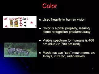
Color. Used heavily in human vision Color is a pixel property, making some recognition problems easy Visible spectrum for humans is 400nm (blue) to 700 nm (red) Machines can “see” much more; ex. X-rays, infrared, radio waves. Imaging Process (review). Factors that Affect Perception.

Color
E N D
Presentation Transcript
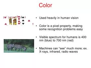
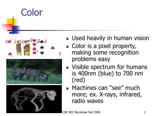
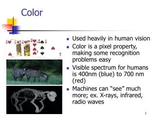
Color • Used heavily in human vision • Color is a pixel property, making some recognition problems easy • Visible spectrum for humans is 400nm (blue) to 700 nm (red) • Machines can “see” much more; ex. X-rays, infrared, radio waves
Factors that Affect Perception • Light: the spectrum of energy that • illuminates the object surface • Reflectance: ratio of reflected light to incoming light • Specularity: highly specular (shiny) vs. matte surface • Distance: distance to the light source • Angle: angle between surface normal and light • source • Sensitivity how sensitive is the sensor
Some physics of color • White light is composed of all visible frequencies (400-700) • Ultraviolet and X-rays are of much smaller wavelength • Infrared and radio waves are of much longer wavelength
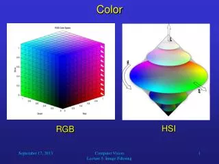
Coding methods for humans • RGB is an additive system (add colors to black) used for displays • CMY[K] is a subtractive system for printing • HSV is good a good perceptual space for art, psychology, and recognition • YIQ used for TV is good for compression
RGB color cube • R, G, B values normalized to (0, 1) interval • human perceives gray for triples on the diagonal • “Pure colors” on corners
Color hexagon for HSI (HSV) Color is coded relative to the diagonal of the color cube. Hue is encoded as an angle, saturation is the relative distance from the diagonal, and intensity is height. intensity saturation hue
Editing saturation of colors (Left) Image of food originating from a digital camera; (center) saturation value of each pixel decreased 20%; (right) saturation value of each pixel increased 40%.
Properties of HSI (HSV) • Separates out intensity I from the coding • Two values (H & S) encode chromaticity • Convenient for designing colors • Hue H is defined by an angle • Saturation S models the purity of the color S=1 for a completely pure or saturated color S=0 for a shade of “gray”
YIQ and YUV for TV signals • Have better compression properties • Luminance Y encoded using more bits than chrominance values I and Q; humans more sensitive to Y than I,Q • NTSC TV uses luminance Y; chrominance values I and Q • Luminance used by black/white TVs • All 3 values used by color TVs • YUV encoding used in some digital video and JPEG and MPEG compression
Conversion from RGB to YIQ We often use this for color to gray-tone conversion.
Colors can be used for image segmentation into regions • Can cluster on color values and pixel locations • Can use connected components and an approximate color criteria to find regions • Can train an algorithm to look for certain colored regions – for example, skin color
Color Clustering by K-means Algorithm Form K-means clusters from a set of n-dimensional vectors 1. Set ic (iteration count) to 1 2. Choose randomly a set of K means m1(1), …, mK(1). 3. For each vector xi, compute D(xi,mk(ic)), k=1,…K and assign xi to the cluster Cj with nearest mean. 4. Increment ic by 1, update the means to get m1(ic),…,mK(ic). 5. Repeat steps 3 and 4 until Ck(ic) = Ck(ic+1) for all k.
K-means Clustering Example Original RGB Image Color Clusters by K-Means
Extracting “white regions” • Program learns white from training set of sample pixels. • Aggregate similar neighbors to form regions. • Components might be classified as characters. • (Work contributed by David Moore.) (Left) input RGB image (Right) output is a labeled image.
Skin color in RGB space Purple region shows skin color samples from several people. Blue and yellow regions show skin in shadow or behind a beard.
Finding a face in video frame • (left) input video frame • (center) pixels classified according to RGB space • (right) largest connected component with aspect similar to a face (all work contributed by Vera Bakic)
Color histograms can represent an image • Histogram is fast and easy to compute. • Size can easily be normalized so that different image histograms can be compared. • Can match color histograms for database query or classification.
Retrieval from image database Top left image is query image. The others are retrieved by having similar color histogram (See Ch 8).
How to make a color histogram • Make 3 histograms and concatenate them • Create a single pseudo color between 0 and 255 by using 3 bits of R, 3 bits of G and 2 bits of B (which bits?) • Can normalize histogram to hold frequencies so that bins total 1.0
Apples versus oranges Separate HSI histograms for apples (left) and oranges (right) used by IBM’s VeggieVision for recognizing produce at the grocery store checkout station (see Ch 16).
Swain and Ballard’s Histogram Matchingfor Color Object Recognition Opponent Encoding: Histograms: 8 x 16 x 16 = 2048 bins Intersection of image histogram and model histogram: Match score is the normalized intersection: • wb = R + G + B • rg = R - G • by = 2B - R - G numbins intersection(h(I),h(M)) = min{h(I)[j],h(M)[j]} j=1 numbins match(h(I),h(M)) = intersection(h(I),h(M)) / h(M)[j] j=1
Models of Reflectance We need to look at models for the physics of illumination and reflection that will 1. help computer vision algorithms extract information about the 3D world, and 2. help computer graphics algorithms render realistic images of model scenes. Physics-based vision is the subarea of computer vision that uses physical models to understand image formation in order to better analyze real-world images.
The Lambertian Model:Diffuse Surface Reflection A diffuse reflecting surface reflects light uniformly in all directions Uniform brightness for all viewpoints of a planar surface.
Specular reflection is highly directional and mirrorlike. R is the ray of reflection V is direction from the surface toward the viewpoint is the shininess parameter
Real specular objects • Chrome car parts are very shiny/mirrorlike • So are glass or ceramic objects • And waxey plant leaves
Phong reflection model • Reasonable realism, reasonable computing • Uses the following components (a) ambient light (b) diffuse reflection component (c ) specular reflection component (d) darkening with distance Components (b), (c ), (d) are summed over all light sources. • Modern computer games use more complicated models.
Phong model for intensity at wavelength lambda at pixel [x,y] ambient diffuse specular
Color Image Analysis with an Intrinsic Reflection Model* • The Problem: • Understand the reflection properties of dielectric materials • (e.g. plastics). • Use them to separate highlights from true color of an object. • Apply this to image segmentation. *Klinker, Shafer, and Kanade, ICCV, 1988
The Dichromatic Reflection Model The light reflected from a point on a dielectric non-uniform material is a mixture of the light reflected from the material surface and that from the material body. incident light exiting surface reflection exiting body reflection N
Let L(,i,e,g) be the total reflected light. wavelength i angle of incident light e angle of emitted light g phase angle Then L(,i,e,g) = L (,i,e,g) + L (,i,e,g) s b s • The surface reflection component L (,i,e,g) appears • as a highlight or gloss. • The body reflection component L (,i,e,g) gives the • characteristic object color. s b
The Dichromatic Reflection Equation L(,i,e,g) = m (i,e,g)c () + m (i,e,g)c () s s b b • c and c are the spectral power distributions • m and m are the geometric scale factors s b s b For RGB images, this reduces to the pixel equation C = [R,G,B] = m C + m C s b s b
Object Shape and Color Variation Assumption: all points on one object depend on the same color vectors c () and c (). Then s b • light mixtures all fall into a dichromatic plane • in color space • light mixtures form a dense color cluster • in this plane
Dichromatic Plane c () s • 2 linear clusters • matte points • highlight points highlight line c () b matte line • The combined color cluster looks like a skewed T. • Skewing angle depends on color difference between • body and surface reflection. • As a heuristic, the highlight starts in the upper 50% • of the matte line.
Color Image Analysis • Color segmentation based on RGB will often find • boundaries along highlights and shadows. • The DRM can be used to better segment. Algorithm: 1. compute initial rough segmentation • compute principal components of color distribution • from small, nonoverlapping image windows. • combine neighboring windows with similar color • distributions into larger regions of locally consistent • color
2. For regions with linear descriptions • approximate c by the first eigenvector of its • color distribution • construct a color cylinder with c as axis and • width a multiple of estimated camera noise • use the cylinder to decide which pixels to • include in the image region • result is a color segmentation that outlines • the matte colors b b
3. Use the skewed T idea to find highlight clusters related to the matte clusters. 4. Use matte plus highlights to form the planar hypothesis. 5. Use the planar hypothesis to grow the matte linear object area into the highlight area. See transparency for experimental results.