Inferential Statistics: Null Hypothesis Testing
Inferential Statistics: Null Hypothesis Testing. HDFS 8200: Research Methods in HDFS (Manfra) Fall 2011. Review. Generate a substantive hypothesis from the following observation made by a child life specialist who teaches infant massage:

Inferential Statistics: Null Hypothesis Testing
E N D
Presentation Transcript
Inferential Statistics: Null Hypothesis Testing HDFS 8200: Research Methods in HDFS (Manfra) Fall 2011
Review • Generate a substantive hypothesis from the following observation made by a child life specialist who teaches infant massage: Karen teaches infant massage to parents. The types of massages that most parents show interest in are related to reducing gas build-up in the intestines—which leads to colic, which leads to crying…and crying is no fun! She teaches three types of strokes: (a) the “water wheel,” (b) the “sun and moon,” and (c) the “I love you.” When revisiting with parents at a later time, she asks how things are going. It is her impression that parents tend to say they use the water wheel more often than the others. Ironically, Karen believes the sun and moon is the most effective stroke for reducing colic-related crying. As such, Karen wants to explore three things in a research project: (1) do parents use one stroke more than another? (2) if so, do parents use one stroke over the other due to ease of use? and (3) is one technique better than another for reducing colic-related crying? • (NOTE: most research projects have more than one question and therefore can have more than one research design.)
Parametric vs. Nonparametric • Parametric – uses sample data to make estimations about the population parameters • Assumes a distribution of data in the population—thus, the same is needed in the sample • Most GLM-based procedures (i.e., those that rely on OLS estimation, like regression or ANOVA) use a diagonal variance-covariance matrix and thus have the assumption of normal distribution and homogeneity of variance (homoscedasticity) • Procedures that use Maximum Likelihood (ML) estimation allow for the variance-covariance matrix to change as prescribed by the researcher—thus, are not limited to these assumptions • Nonparametric – does not estimate population parameters • Usually frequency/count data or poorly distributed data
Null hypothesis significance testing • Reformulate the general (substantive wording) hypothesis into two mathematical statements or hypotheses: • null hypothesis (H0) • alternative hypothesis (H1) • These should always be written in terms of the population parameters NOT the sample statistics when conducting parametric tests • Goal is to make inferences about the population parameters; therefore, we establish hypotheses based on what we believe happens in the population (i.e., truth)
Null Hypothesis • The null hypothesis, by definition, means that there is nodifference (0) between different groups of a single populations or no relation among constructs within a given population • NOTE: there is an implicit assumption that the null hypothesis is true; null hypothesis testing merely provides information about whether the collected data is from the same population in which no difference would exist • Example of how to write hypotheses: • H0: µI = µC or µI - µC = 0 • H1: µI > µC or µI - µC > 0 • H1: µI < µC or µI - µC < 0 • Intervention group mean (µI) and control group mean (µC) • NOTE: this can be any population parameter, including correlation coefficients (ρ) or regression weights (β)
Null vs. Alternative • As the name implies, null hypothesis significance testing only explores whether or not the data match or fit the null hypothesis • The alternative hypothesis is NEVER explored with collected data • We “never” know what the true population parameters are (in the rare cases in which we have a good guess at what they are, we set up the null hypothesis to reflect these parameters, called a non-nil null hypothesis; still we only explore the null hypothesis with our data) • This is why we want to minimize the alternatives to the null hypothesis through good study design (important in nonexperimental designs) • This is also why we only use the following terminology when drawing conclusions based on null hypothesis testing: • We reject the null hypothesis when a non-difference cannot be reasonably substantiated (note the double negative) • We fail to reject the null hypothesis when a non-difference can reasonably be substantiated
Alternative Hypotheses • Alternative hypothesis—while NEVER explored statistically—can be expressed as directional or nondirectional • This choice has consequences for the amount of allowed α (Type I error; “significance level”; .05) in the null hypothesis test
Directional vs. Nondirectional • Directional alternative hypotheses specify how the population parameters will behavior in reference to each other • H1: µI - µC > 0 or µI > µC • This puts all the “eggs in one basket” so to speak and allows you to put all of the α (.05) at one-tail of your statistical distribution • Nondirectional alternative hypotheses specify that there will be a difference between the parameters but don’t specify what that difference is • H1: µI - µC ≠ 0 or µI ≠ µC • Because you are not specifying a direction, you have to split your “eggs” so to speak and allow for the possibility of finding an effect at both ends of the statistical distribution • In other words, you have to put half of the α at one-tail (.025) and half at the other side; thus, your power to detect an effect is reduced • NOTE: Most statistical packages assume a two-tailed (nondirectional) hypothesis and many don’t allow the user to adjust or change this
Example Hypotheses • Let’s consider some hypotheses for different research scenarios: • True experimental design with two groups post-test only: H0: µI - µC = 0 H1: µI - µC ≠ 0 • True experimental design with two groups pre-post test design: H0: (µPostI - µPreI) – (µPostC - µPreC) = 0 H1: (µPostI - µPreI) – (µPostC - µPreC) ≠ 0 • Nonexperimental association design: H0: ρAB = 0 H1: |ρAB| > 0 or H1: ρAB ≠ 0 • One-group post-test design**: H0: µ = 0 H1: µ ≠ 0
EXERCISE • If the researcher knows—from previous research—that an affluent population will improve by an average of 15 points after a 3-week intervention and the research wants to specify a null hypothesis to test whether the newly collected data from an impoverished population will improve by the same amount (after the same 3-week intervention), how would s/he write this non-nil null hypothesis? • And an alternative hypothesis? • (NOTE: s/he will only collected data from the impoverished population for this study.)
Test Review Redux • Take the substantive hypothesis you generated at the beginning of class and write out the null hypothesis and an alternative hypothesis • What are the variables of interest? • What type of design would you use to address each question?
THOUGHT QUESTIONS • Why is it useful to explore/test the null hypothesis? Look back at the null hypotheses, what do researchers need (or not need) to know with this approach to statistical testing? (HINT: it is a mathematical factor.) • Substantively, what is the null hypothesis really saying? • It is saying that the two groups in your study (I and C) are from the same population. If you reject this hypothesis, then you are saying that the two groups are from different populations. • The process of null hypothesis testing is really getting at whether or not you can reliably (based on probabilities) state that data you collected come from the same, or not the same, population. Or, in the case of single sample designs, whether or not the data you collected comes from the population of interest. • What is an example of when the null hypothesis is the hypothesis of interest to the researcher (i.e., the research hypothesis)?
Error in Null Hypothesis Testing • Type I error (α) – reject the null hypothesis, when it is true • This is the more dangerous error…meaning, a researcher might change a curriculum in a school or an intervention in an alcohol treatment program, when the curriculum or the intervention actually do not work • Typically set a priori and very common to have discipline standards • Most social scientists set the acceptable level of Type I error at .05 (i.e., α = .05) • Hence, we look for the probability of a Type I error to be less than .05 (i.e., p < .05)
Error in Null Hypothesis Testing • Type II error (β) – fail to reject the null hypothesis, when it is false • This is less dangerous…there actually is a difference but you failed to find one • This happens all the time! • While the Type I error (or α) is preset at .05, the Type II error depends on the amount of power in your study and therefore can vary greatly between studies • NOTE: power = 1 – β (Type II error) • Low power—perhaps caused by a small sample size—can lead to Type II error
Why use Null Hypothesis Testing? • Many good arguments against using null hypothesis testing (see pp. 240-242)—be sure to know why we use it • Answers to thought question: • comes down to the simplicity of making a known out of an unknown! • The whole point of conducting research and estimating population parameters with sample statistics is because we do not know what the population parameters are • If we don’t know the population parameters, how do we test whether or not our statistical values are good estimates of the population parameters? • Simple…we manipulate our population parameters and set them at a theoretically known value…like 0.
Why the Null Hypothesis? • But, how can zero (0) be a known value if everything in population is unknown? • Assume everyone (men and women) in a theoretical population has a mean of 30 on a given measure. • This means that men have a mean of 30 and women have a mean of 30. • If you take the difference between men and women (the two groups of interest), we get 30 – 30 or 0. • Therefore, it doesn’t matter what the mean is of the two groups, if we assume they are from the same population and thus have the same value, then their difference has to equal 0. • Hence, we don’t really have to worry about the actual value of the population. • Null testing doesn’t ever tell us what the actual population parameter is…just that it isn’t zero (0)
Data Analysis Choice • Three general rules of thumb: • Use the most parsimonious (correct) procedure for the job • No need to use a Mixed Model to analyze data when a t-test can be used • Use the correct procedures that are common within the research community (i.e., what others are using in the journals in which you wish to publish) • Use the correct procedures that are most comfortable to you and that you have the most confidence conducting • If you are conducting multiple analyses in which you are adding or subtracting variables, it is best to use the same procedure if possible for all tests (e.g., use ANOVA even when exploring one variable with two-levels)
GLM Equations for Common Tests • Independent samples t-test: • y = b0 + b1x • where b1 represents the mean difference between levels; significance is based on whether b1 is not equal to zero (0) • Correlation: • y = B1x • where B1 is the standardized coefficient of variation between x and y (NOTE: y-intercept is set to 0 when standardized); significance is based on whether B1 is non-zero • One-way (IV: 3 discrete levels) ANOVA: • y = b0 + b1x1 + b2x2 • where b1 represents the difference between level 0 and level 1 and b2 represents the difference between level 0 and level 2; significance is based on whether b1 and/or b2 are non-zero
GLM Equations for Common Tests • Two-way (GROUP: 2 levels) repeated measures (TIME: 2 levels) ANOVA (factorial): • y = b0 + b1GROUP + b2TIME + b3GROUP*TIME • where b3 represents the interaction effect between GROUP and TIME • Multivariate Regression (2 continuous IVs: STRESS and DAYS): • y = b0 + b1STRESS + b2DAYS
EXAMPLE W/ SPSS OUTPUT • Do people who go to graduate school have less test anxiety compared to those who do not go to graduate school? • H0: µGRAD_YES - µGRAD_NO = 0 • H1: µGRAD_YES - µGRAD_NO > 0 • Is this directional or nondirectional? One-tail or two-tail test?? • Goal: Compare means of two groups (Gradschool_YES and Gradschool_NO)
Test Anxiety (M) No (0) Yes (1) Gradschool? Test Anxiety (M) No (0) Yes (1) Gradschool? EXAMPLE W/ SPSS OUTPUT • Goal: Compare means of two groups (Gradschool_YES and Gradschool_NO) • H0 and H1 drawn out graphically • Equation to test model: Y = B0 + B1GRADSCHOOL Recall, B1 is the slope of the dotted line in the graphs. If B1 is zero (0)—H0--, then we fail to reject the null hypothesis; if B1 is significantly above zero (0)—H1--, then we reject the null hypothesis. H1 H0
EXAMPLE W/ SPSS OUTPUT • Appropriate statistical tests • Based on the graphical representation, any general linear model will be able to test for the desired effect • Two-samples (independent samples) t-test, ANOVA, regression, point-biserial correlation • Easier (less time consuming) to do hand calculations for t-tests and ANOVAs • In all cases, the statistical value (whether t or F) will provide information about whether you should reject or fail to reject the null hypothesis • Output is based on fictitious file: SPSSExamples1.sav
EXAMPLE W/ SPSS OUTPUT Note the mean difference between the two groups is 3.84, which is greater than 0. Is it statistically significant? Output from independent t-test is below. The t value is the test statistic, the Sig (2-tailed) is p value. (Note: 2-tailed output not 1-tailed) The mean difference is statistically significant.
EXAMPLE W/ SPSS OUTPUT The approach of ANOVA is different than a t test in how the variance is parsed. ANOVA divides variance into between group and within group variance and then proceeds to calculate an F value. t-test is calculated by mean difference and standard error comparison. BUT, same result!! t value squared = F value 18.6915391102443562 = 349.3736343 ~= 349.374
EXAMPLE W/ SPSS OUTPUT Regression Output: This is the B0 value—or y-intercept. Note it is the same value as the group that is equal to 0 (i.e., gradschool_no) What do you think this is? This is B1—note it is exactly the same as mean difference in t-test—difference between gradschool_no (0) and gradschool_yes (1)
EXAMPLE W/ SPSS OUTPUT Though mathematically the same as a Pearson Correlation, this is called a Point-Biserial Correlation because one variable is dichotomous and one variable is continuous (Pearson uses two continuous variables).
Test Scenario • Does undergraduate ranking relate to math scores? • Use SPSSExample1.sav file