Download

1 / 161
1.66k likes | 1.92k Views
SAA 2023 COMPUTATIONALTECHNIQUE FOR BIOSTATISTICS. Inferential Statistics. Inferential Statistics. Computational Statistics: - All you need to do is choose statistic - Computer does all other steps for you!!!!!!. Inferential Statistics. Inferential Statistics. Inferential Statistics.

E N D
SAA 2023 COMPUTATIONALTECHNIQUE FOR BIOSTATISTICS Inferential Statistics
Inferential Statistics Computational Statistics: - All you need to do is choose statistic - Computer does all other steps for you!!!!!!
Inferential Statistics For instance, if I am asked by a layperson what is meant exactly by statistics, I will refer to the following Old Persian saying: “Mosht Nemouneyeh Kharvar Ast (translated: a handful represents the heap).
Inferential Statistics This brief statement will describe, in one sentence, the general concept of inferential statistics. In other words, learning about a population by studying a randomly chosen sample from that particular population can be explained by using an analogy similar to this one.
Inferential Statistics • Involves using obtained sample statistics to estimate the corresponding population parameters • Most common inference is using a sample mean to estimate a population mean (surveys, opinion polls) • Drawing conclusions from sample to population • Sample should be representative
Inferential Statistics • Inferential statistics allow us to make determinations about whether groups are significantly different from each other.
Inferential Statistics Inferential statistics is not a system of magic and trick mirrors. Inferential statistics are based on the concepts of probability (what is likely to occur) and the idea that data distribute normally
Sample of observations Entire population of observations Random selection Parameter µ=? Statistic Statistical inference
Inferential Statistics Inferential statistics is based on a strange and mystical concept called falsification. Although you might think the process is simple Write a hypothesis, test it, hope to prove it Inferential statistics works this way:
Inferential Statistics Write a hypothesis you believe to be true. Write the OPPOSITE of this hypothesis, which is called the null hypothesis. Test the null, hoping to reject it. • If the null is rejected, you have evidence that the hypothesis you believe to be true may be true. • If the null is failed to reject, reach no conclusion.
Inferential Statistics Two major sources of error in research Inferential statistics are used to make generalizations from a sample to a population. There are two sources of error (described in the Sampling module) that may result in a sample's being different from (not representative of) the population from which it is drawn. These are: Sampling error - chance, random error Sample bias - constant error, due to inadequate design
Inferential Statistics Inferential statistics take into account sampling error. These statistics do not correct for sample bias. That is a research design issue. Inferential statistics only address random error (chance). Sampling error - chance, random error Sample bias - constant error, due to inadequate design
Inferential Statistics p-value The reason for calculating an inferential statistic is to get a p-value (p = probability). The p value is the probability that the samples are from the same population with regard to the dependent variable (outcome). Usually, the hypothesis we are testing is that the samples (groups) differ on the outcome. The p- value is directly related to the null hypothesis.
Inferential Statistics The p-value determines whether or not we reject the null hypothesis. We use it to estimate whether or not we think the null hypothesis is true. The p-value provides an estimate of how often we would get the obtained result by chance, if in fact the null hypothesis were true.
Inferential Statistics If the p-value (< α- value) is small, reject the null hypothesis and accept that the samples are truly different with regard to the outcome. If the p-value (> α- value) is large, fail to reject the null hypothesis and conclude that the treatment or the predictor variable had no effect on the outcome.
Inferential Statistics Steps for testing hypotheses • Calculate descriptive statistics • Calculate an inferential statistic • Find its probability (p-value) • Based on p-value, accept or reject the null hypothesis (H0) • Draw conclusion
Inferential Statistics One-Sample T: GPAs Variable N Mean StDev SE Mean 90% CI GPAs 50 2,9580 0,4101 0,0580 (2,8608; 3,0552) Variable N Mean StDev SE Mean 95% CI GPAs 50 2,9580 0,4101 0,0580 (2,8414; 3,0746) • Sample mean = 2,96 • - 90% confident that μ(population mean) is between 2,86 and 3,06 • 95% confident that μ(population mean) is between 2,84 and 3,07 • 95% CI width > 90% CI width • The larger confidence coefficient, the greater the CI width
Inferential Statistics One-Sample T: GPAs Test of μ = 3 vs < 3 (directional, one-tail to the right) 95% Upper Variable N Mean StDev SE Mean Bound T P GPAs 50 2,9580 0,4101 0,0580 3,0552 -0,72 0,236 Test of μ = 3 vs ≠ 3 (non-directional, two-tail) Variable N Mean StDev SE Mean 95% CI T P GPAs 50 2,9580 0,4101 0,0580 (2,8414; 3,0746) -0,72 0,472 Test of μ = 3 vs > 3 (directional, one-tail to the left) 95% Lower Variable N Mean StDev SE Mean Bound T P GPAs 50 2,9580 0,4101 0,0580 2,8608 -0,72 0,764
Inferential Statistics One-Sample T: GPAs Test of μ = 3 vs < 3 95% Upper Variable N Mean StDev SE Mean Bound T P GPAs 50 2,9580 0,4101 0,0580 3,0552 -0,72 0,236 The test statistic, t = -0,72, is the number of std deviations that the sample mean 2,96 is from the hypothesized mean, μ = 3. p-value is the probability that a random sample mean is less than or equal to 2,96 when Ho: μ = 3 is true. The rejection region consists of all p-values less than α. p-value = 0,236 > α = 0,05 Then, we fail to reject Ho Conclusion: There is not sufficient evidence in the sample to conclude that the true mean GPA, μ, is less than 3.00.
Inferential Statistics Two sample T-test
Inferential Statistics Non-directional (2-tailed test): In this form of the test, departure can be observed from either end of the distribution. Thus, no direction for expected results are specified. The null and alternative hypotheses are as follows: Directional (1-tailed test): In this form of the test, the rejection region lies at only one end of the distribution. The direction is specified before any analysis begins.
One-sample t-test Cholesterol Example: Suppose population mean μ is 211 = 220 mg/ml s = 38.6 mg/ml n = 25 (town) H0 : m = 211 mg/ml HA : m ¹ 211 mg/ml For an a = 0.05 test we use the critical value determined from the t(24) distribution. Since |t| = 1.17 < 2.064 (table t) at the a = 0.05 level We fail to reject H0. The difference is not statistically significant
One-sample t-test • We set a standard beyond which results would be rare (outside the expected sampling error) • We observe a sample and infer information aboutthe population • If the observation is outside the standard, we rejectthe hypothesis that the sample is representative of the population