Download
1 / 38
380 likes | 502 Views
The Most General Markov Substitution Model on an Unrooted Tree. Von Bing Yap Department of Statistics and Applied Probability National University of Singapore Acknowledgements: Rongli Zhang, Lior Pachter. Statistical Phylogenetics.

E N D
The Most General Markov Substitution Model on an Unrooted Tree Von Bing Yap Department of Statistics and Applied Probability National University of Singapore Acknowledgements: Rongli Zhang, Lior Pachter
Statistical Phylogenetics • Neyman (1971): phylogenetics can be formulated as an inference problem, where the unknown parameters are (1) tree topology (primary) (2) evolution process (“nuisance”)
Methods in framework • Maximum likelihood • Bayesian to a lesser extent • Parsimony • Distance
Stochastic Models • In almost all substitution models used, the transition probabilities are generated from (1) a reversible rate matrix (REV or special case) or (2) a family of reversible rate matrices (Yang and Roberts 1985, Galtier and Gouy 1998)
Special vs General • The choice between simple and general model is a trade-off between bias and variance. • Simple: smaller variance in estimates, larger bias. • General: larger variance in estimates, smaller bias.
The case for general models • The tree parameter space, unlike the process parameters, is unchanged, so the bias-variance trade-off maybe less of an issue. • It is plausible that general models may get the right tree more often.
Binary Unrooted Trees • An (unrooted) tree where all internal nodes are of degree 3. • Such a tree arises from a rooted binary tree where the root has degree 2.
General Markov Process • Pick any node in an unrooted tree as the “root”. All edges become directed. • Parameters: base frequency at root transition probability matrix Pab for the directed edge going from node a to node b.
Alternative Views • Picking another node as the root, and appropriate parameter values, can give the same joint distribution at all nodes. • This is a Markov random field, which can be viewed as a Markov process in many ways.
Same as before, if diag(π0) P01 = t(P10) diag(π1)
Identifiability • Chang (1996): if root base frequencies are all positive, all transition probabilities are invertible and diagonal dominant, then parameters are uniquely determined by the joint distribution at leaf nodes.
Inference • Given an unrooted tree, find the most likely process. The loglikelihood is the support for the tree. • Choose the tree with the highest support. • Likelihood of data computed with Felsenstein’s algorithm.
Parameter Estimation on Fixed Tree • Case 1: all node states are observed • Case 2: only leaf node states are observed
Case 1: all node states observed • Pick a root node. • The base frequencies at root are estimated by the observed frequencies. • For each directed edge, the transition probability is obtained by dividing the frequency table of changes by the row sums. • These are MLEs.
π0 estimated from base composition of sequence 0. Three frequency tables: F01 for going from 0 to 1, F02, and F03. P01 estimated by dividing each row of F01 by sum; etc ….
Case 2: only leaf node states observed • Root sequence and all frequency tables are unknown, so are random variables under the model. • Let θ0 be a set of parameter estimates. Find conditional expectation of root sequence and frequency tables, given leaf sequences, under θ0.
Put π0, P01, P02 and P03 as determined by θ0. Find conditional expectation of sequence 0 and frequency tables F01, F02 and F03 under these parameters, given the observed data.
Case 2 (continued) • Problem reduced to Case 1, with unobserved root sequence and frequency tables replaced by conditional expectations, the imputed data. • Applying Case 1 gives a new set of parameter estimates θ1.
EM algorithm • Start with an initial parameter estimate θ0. • E-step: find conditional expectation of the root sequence and frequency tables, given leaf sequences, under model θ0.
EM algorithm • M-step: find MLE θ1 based on the imputed data. • Iterate the process to get θ2, θ3 … The likelihoods are guaranteed to increase and converge to a local maximum (Baum 1973, Rubin et al 1977).
Applications • Simulated sequences with Jukes-Cantor model • Simulated sequences with Felsenstein’s example • Phylogeny of human, mouse, dog and chicken
Sidall (1998) • In 4-taxon simulation studies using Jukes-Cantor model, parsimony outperforms ML analysis based on Jukes-Cantor and even general reversible (REV) models.
t and z are equal and moderate small t, large z
Felsenstein (1983)
π = (1–RR) P1 (row 1) = (1–QQ) P1 (row 2) = ( 0 1) P2 (row 1) = (1–PP) P2 (row 2) = ( 0 1)
Not a usual model • The equilibrium distribution of the transition matrices is (0 1): eventually all states become 1. • Still fits in the present framework.
Reconstruction • Someone simulates sequences with some R, Q, P values hidden from you. • You are asked to reconstruct the tree: 3 possibilities.
f f e f e e f f f e e e Using the usual models, how much information should be put in? Should the branches e have the same length, and f have the same length? Seems unnatural, and may be unfair to some possibilities.
Fit General Model • Simulation results: percentage accuracy for R = 0.20, Q = 0.10, P = 0.35:
Tree 1: human and dog are sister taxa Tree 2: human and mouse are sister taxa
Comparison of Trees • Data: ~40,000 4D sites from the CFTR region from Lior Pachter • 6 analyses: all, first 1/5, next 1/5,… • All analyses support Tree 1 over Tree 2.
Discussion • The General Markov process is simple to imagine and to estimate. • No explicit branch lengths. Approximate lengths possible. • No natural way of incorporating site heterogeneity.