Download
1 / 34
340 likes | 362 Views
A polarizable QM/MM model for the global (H 2 O) N – potential surface. John M. Herbert Department of Chemistry Ohio State University. IMA Workshop “Chemical Dynamics: Challenges & Approaches” Minneapolis, MN January 12, 2009. $$. B.B.G. 2006. CAREER. Acknowledgements.

E N D
A polarizable QM/MM model for the global (H2O)N– potential surface John M. Herbert Department of Chemistry Ohio State University IMA Workshop “Chemical Dynamics: Challenges & Approaches” Minneapolis, MN January 12, 2009
$$ B.B.G. 2006 CAREER Acknowledgements Group members: Dr. Mary Rohrdanz Dr. Chris Williams Leif Jacobson Adrian Lange Ryan Richard Katie Martins Mark Hilkert Dr. Chris Williams Leif Jacobson
n 100 30 15 200 50 20 11 6 2 0.0 ? -0.5 -1.0 -1.5 -2.0 Neumark -2.5 -3.0 – VDE / eV = –3.30 + 5.73 n–1/3 -3.5 1.0 0.0 0.2 0.4 0.6 0.8 (H2O)n– vertical electron binding energies (VEBEs) Isomer I Isomer I VDE / eV – VDE (eV) VEBE / eV —VEBE / eV Experiments Johnson n n I Experiment: Abrupt changes atn = 11and n = 25 followed by smooth (?) extrapolation Johnson: CPL 297, 90 (1998) JCP 110, 6268 (1999) Coe/Bowen: JCP 92, 3980 (1990) Neumark: Science 307, 93 (2005) n-1/3 n -1/3
n 100 30 15 200 50 20 11 6 2 0.0 ? III -0.5 -1.0 II -1.5 -2.0 Theory (1980s): Surface to internal transition occurs between n = 32 and n = 64 Neumark -2.5 -3.0 -3.5 1.0 0.0 0.2 0.4 0.6 0.8 Simulations: Barnett, Landman, Jorter JCP 88, 4429 (1988) CPL 145, 382 (1988) (H2O)n– vertical electron binding energies (VEBEs) – VDE (eV) —VEBE / eV Experiments Johnson I Simulation: Internal Surface n-1/3 n -1/3
expt. Turi & Borgis, JCP 117, 6186 (2002) Interior (cavity) states are stable only for T ≤ 100 K or n ≥ 200 J.V. Coe et al. Int. Rev. Phys. Chem. 27, 27 (2008) Theory (21st century version) simulated absorption spectra for (H2O)N– Turi & Rossky, Science 309, 914 (2005)
V(anion) V(neut) VEBE E(neut) E(anion) Global minima Importance of the neutralwater potential for water cluster anions
(H2O)20– isomers VEBE = 0.42 eV E(anion) = 0.00 eV E(neut) = 0.45 eV V(anion) V(neut) VEBE = 0.39 eV E(anion) = 0.01 eV E(neut) = 0.43 eV VEBE E(neut) E(anion) VEBE = 0.72 eV E(anion) = 0.03 eV E(neut) = 0.78 eV Global minima
e– correlation is more important for cavity states correlation strength vs. e– binding motif VEBE (eV) ∆ = Ecorr(anion) - Ecorr(neutral) (eV) C.F. Williams & JMH, J. Phys. Chem. A112, 6171 (2008)
e– correlation is more important for cavity states correlation strength vs. e– binding motif surface states VEBE (eV) ∆ = Ecorr(anion) - Ecorr(neutral) (eV) C.F. Williams & JMH, J. Phys. Chem. A112, 6171 (2008)
e– correlation is more important for cavity states correlation strength vs. e– binding motif cavity states VEBE (eV) ∆ = Ecorr(anion) - Ecorr(neutral) (eV) C.F. Williams & JMH, J. Phys. Chem. A112, 6171 (2008)
Motivation for the new model • The electron–water interaction potential has been analyzed carefully, but almost always used in conjunction with simple, non-polarizable water models (e.g., Simple Point Charge model, SPC). • L. Turi & D. Borgis, J. Chem. Phys. 114, 7805 (2001); 117, 6186 (2002) • A QM treatment of electron–water dispersion via QM Drude oscillators provides ab initio quality VEBEs, but requires expensive many-body QM • F. Wang, T. Sommerfeld, K. Jordan, e.g.: J. Chem. Phys. 116, 6973 (2002) J. Phys. Chem. A 109, 11531 (2005) • How far can we get with one-electron QM, using a polarizable water model that performs well for neutral water clusters? • AMOEBA water model: P. Ren & J. Ponder, J. Phys. Chem. B 107, 5933 (2003)
(H2O)– wavefn. O H H nodeless pseudo-wavefn. Electron–water pseudopotential 1) Construct a repulsive effective core potential representing the H2O molecular orbitals:
(H2O)– wavefn. O H H nodeless pseudo-wavefn. Electron–water pseudopotential 1) Construct a repulsive effective core potential representing the H2O molecular orbitals: 2) Use a density functional form for exchange attraction, e.g., the local density (electron gas) approximation: 3) In practice these two functionals are fit simultaneously
AMOEBA electrostatics Define multipole polytensors and interaction polytensors where i and j index MM atomic sites and Then the double Taylor series that defines the multipole expansion of the Coulomb interaction can be expressed as
Polarization * In AMOEBA, polarization is represented via a linear-response dipole at each MM site: The total electrostatic interaction, including polarization, is where *P. Ren & J.W. Ponder, J. Phys. Chem. B 127, 5933 (2003)
Polarization work The electric field at MM site i is Some work is required to polarize the dipole in the presence of the field: So the total electrostatic interaction is really
Electron–multipole interactions To avoid a “polarization catastrophe” at short range, we employ a damped Coulomb interaction:
Recovering a pairwise polarization model In general within our model we have: Imagine instead that each H2O has a single, isotropic polarizable dipole whose value is induced solely by qelec: Then the electron–water polarization interaction is In practice we use an attenuated Coulomb potential, the effect of which can be mimicked by an offset in the electron–water distance: This is a standard ad hoc polarization potential that has been used in may previous simulations.
Fourier Grid Simulations • Simultaneous solution of where i = 1, ..., NMM. cI= vector of grid amplitudes for the wave function of the Ith electronic state H depends on the induced dipoles. • Solution of the linear-response dipole equation is done via iterative matrix • operations. Dynamical propagation of the dipoles (i.e., an extended- • Lagrangian approach) is another possibility. • Solution of the Schrödinger equation is accomplished via Fourier grid • method using a modified Davidson algorithm (periodically re-polarize the • subspace vectors) • The method is fully variational provided that all polarization is done self-consistently
34 clusters from N=2 to N=19 75 clusters from N=20 to N=35 Model VEBE / eV Ab initio VEBE / eV Vertical e– binding energies for (H2O)N– Exchange/repulsion fit to (H2O)2– VEBE Non-polarizable model: Turi & Borgis, J. Chem. Phys. 117, 6186 (2002)
34 clusters from N=2 to N=19 75 clusters from N=20 to N=35 Model VEBE / eV Ab initio VEBE / eV Vertical e– binding energies for (H2O)N– Exchange/repulsion fit to entire database of VEBEs Non-polarizable model: Turi & Borgis, J. Chem. Phys. 117, 6186 (2002)
Analysis electron–water polarization (kcal/mol)
e– correlation is more important for cavity states correlation strength vs. e– binding motif surface states, n = 2–24 DFT geometries VEBE (eV) ∆ = Ecorr(anion) - Ecorr(neutral) (eV) C.F. Williams & JMH, J. Phys. Chem. A112, 6171 (2008)
e– correlation is more important for cavity states correlation strength vs. e– binding motif surface states, n = 2–24 DFT geometries VEBE (eV) ∆ = Ecorr(anion) - Ecorr(neutral) (eV) C.F. Williams & JMH, J. Phys. Chem. A112, 6171 (2008)
surface states, n = 18–22 model Hamiltonian geometries e– correlation is more important for cavity states correlation strength vs. e– binding motif VEBE (eV) ∆ = Ecorr(anion) - Ecorr(neutral) (eV) C.F. Williams & JMH, J. Phys. Chem. A112, 6171 (2008)
cavity states, n = 28–34 model Hamiltonian geometries e– correlation is more important for cavity states correlation strength vs. e– binding motif VEBE (eV) ∆ = Ecorr(anion) - Ecorr(neutral) (eV) C.F. Williams & JMH, J. Phys. Chem. A112, 6171 (2008)
e– correlation is more important for cavity states correlation strength vs. e– binding motif cavity states, n = 14, 24 DFT geometries VEBE (eV) ∆ = Ecorr(anion) - Ecorr(neutral) (eV) C.F. Williams & JMH, J. Phys. Chem. A112, 6171 (2008)
0.6 0.5 cavity state, VEBE = 0.58 eV surface state, VEBE = 0.87 eV mainly just a bunch of weak interactions 0.4 0.3 0.2 0.1 fraction of total pairs many stronger correlations 1 1 3 3 5 5 7 7 9 9 11 11 13 13 15 15 17 17 19 19 Quantifying electron–water dispersion SOMO pair correlation energy / meV C.F. Williams & JMH, J. Phys. Chem. A112, 6171 (2008)
water– water e––water electrostatics fit to exchange/ repulsion Putting it all together: