Bayesian Network Representation Explained
Explore the mathematical foundation of Bayesian networks and the parameterization of joint distributions. Understand how to represent independent random variables and conditional probabilities using Bayesian models.

Bayesian Network Representation Explained
E N D
Presentation Transcript
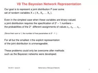
V8 The Bayesian Network Representation Ourgoalistorepresent a jointdistribution P oversome setofrandom variables X = { X1, X2, …Xn }. Even in thesimplestcasewhenthese variables arebinary-valued, a jointdistributionrequiresthespecificationof 2n – 1 numbers – theprobabilitiesofthe2n different assignmentsofvalues x1, x2, … xn . (Sincetheirsumis 1, thenumberoffreeparametersis 2n - 1 .) For all but thesmallestnthe explicit representation ofthejointdistributionisunmanageable. These problemscouldonlybeovercome after methods such astheBayesiannetworksweredeveloped. Mathematics of Biological Networks
Independent Random Variables Letusstartbyconsidering a simple settingwereweknow thateachXirepresentstheoutcomeof a tossofcoini. Wetypicallyassumethatthe different cointossesaremarginally independent, so thatthedistribution P will satisfy (XiXj ) foranyi, j. More generallyweassumethatthedistributionsatisfies (XY) foranydisjointsubsetsofthe variables XandY. Therefore P(X1, X2, … Xn) = P(X1) P(X2) … P(Xn) Ifweusethestandardrepresentationofthejointdistribution, thisindependencestructureisobscuredandtherepresentation requires2nparameters. Mathematics of Biological Networks
Independent Random Variables However, wecanuse a morenaturalsetofparameters forspecifyingthisdistribution. If iistheprobabilitywithwhichcoinilandsheads, thejointdistributionPcanbespecifiedusingthenparameters1… n . These parametersimplicitlyspecifythe2nprobabilities in thejointdistribution. Forexample, theprobabilitythat all ofthecointosseslandheadsissimply 1 2 … n . More generally, lettingwhen and when wecandefine (This meansthatwehaveusedforeachcointhefactthattheprobabilitiesneedtosumupto 1). Mathematics of Biological Networks
Independent Random Variables This representationis limited, andtherearemanydistributions thatwecannotcapturebychoosingvaluesfor 1… n . This isquiteobviousbecausethespaceof all jointdistributionsis (2n -1 )- dimensional andwecan in general not coverthisby an n–dimensional manifold. This onlyworked in thiscaseofnindependentrandom variables. Mathematics of Biological Networks
Conditionalparametrization Considertheproblemfacedby a companytrying tohire a recentcollegegraduate. The company‘sgoalistohire intelligent employees, but thereisnowaytotestintelligencedirectly. Let‘sassumethatthecompanyhasaccesstothestudent‘s SAT score. Ourprobabilityspaceisnowinducedbythetworandom variables Intelligence (I) and SAT (S). Forsimplicity, weassumethateachofthesetakes 2 values: - Val(I) = { i1 , i0 } whichrepresenthighandlowintelligence - Val(S) = { s1, s0 } whichrepresentthevalueshighandlow score. Mathematics of Biological Networks
Conditionalparametrization The jointdistributionhas 4 entries. E.g. Thereis an alternative andmorenaturalwayofrepresentingthe same jointdistribution. Usingthechainruleofconditionalprobabiliteswehave Thus, insteadofspecifyingthevariousjointentries P(I,S), wecanspecifyit in the form of P(I) and P(S|I). Mathematics of Biological Networks
Conditionalparametrization E.g. wecanrepresentthepreviousjointdistributionbythefollowing 2 tables, onerepresentingthepriordistributionover I andtheother theconditionalprobabilitydistribution (CPD) of S given I: Thus, a studentoflowintelligenceisveryunlikelytoget a high SAT score (P (s1| i0) = 0.05). On theotherhand, a studentof high intelligencehas a goodchance toget a high SAT score (P (s1 | i1) = 0.8) but thisis not certain. Mathematics of Biological Networks
Conditionalparametrization Howcanweparametrizethis alternative representation? Here, weareusing 3 binomialdistributions, onefor P(I), and 2 for P(S|i0) andP(S| i1). Wecanparametrizethisrepresentationusing 3 independentparameters. Ourrepresentationofthejointdistributionas a 4-outcome multinomial also required 3 parameters. → The newrepresentationis not morecompact. The figure on therightshowsfig. 3.1.a a simple Bayesiannetwork forthisexample. Eachofthe 2 random variables I and S has a node, andtheedgefrom I to S representsthedirection ofdependence in thismodel. Mathematics of Biological Networks
The studentexample: new variable grade We will nowassumethatthecompany also hasaccess tothestudent‘sgrade G in somecourse. Then, ourprobabilityspaceisthejointdistributionofthe 3 relevant random variables I, S, and G. Assuming I and S asbeforeand G takes on 3 valuesg1, g2, g3representing the grades A, B and C, respectively.The jointdistributionhas 12 entries. In thiscase, independence (of variables) does not help. The student‘sintelligenceisclearlycorrelatedboth withhis/her SAT score andhis/her grade. The SAT score is also correlatedwiththe grade. Mathematics of Biological Networks
The naive Bayesmodel Weexpectthatforourdistribution P P( g1|s1 ) > P(g1 | s0) However, itisquite plausible thatourdistribution P satisfies a conditionalindependenceproperty: Ifweknowthatthestudenthas high intelligence, a high grade on the SAT nolongergivesusinformationaboutthestudent‘sperformance in theclass. P( g | i1 ,s1) = P(g| i1) More generally, wemaywellassumethat P |= (S G | I) This independencestatementonlyholdsifweassume thatthestudent‘sintelligenceistheonlyreason whyhis/her grade and SAT score mightbecorrelated. Mathematics of Biological Networks
The naive Bayesmodel By simple probabilisticreasoningwe also havethat P(I,S,G) = P(S,G | I) P(I) The previouseq. P |= (S G | I) impliesthat P(S,G | I) = P(S | I) P(G | I) Hence, weget P(I,S,G) = P(S | I) P(G | I) P(I) Thus, wehavefactorizedthejointdistribution P(I,S,G) as a productof 3 conditionalprobabilitydistributions(CPDs). P(I) and P(S | I) canbere-usedfrom p.7. P(G | I) could, e.g., havethe following form Mathematics of Biological Networks
The naive Bayesmodel Together, these 3 CPDs fullyspecifythejointdistribution (assumingP |= (S G | I) ). Forexample P(i1, s1, g2 ) = P(i1 ) P(s1 | i1 ) P(g2 | i1 ) = 0.3 0.8 0.17 = 0.0408 This probabilisticmodelisrepresentedusingtheBayesiannetworkshownbelow. In thiscase, the alternative parametrization ismorecompactthanthejoint. The 3 binomialdistributions P(I), P(S | i1) and P(S | i0) require 1 parametereach. The 3-valued multinomialdistributionsP(G | i1) and P(G | i0) require 2 parameterseach. This makes 7 parameters, comparedtotheAnotheradvantageisthe jointdistributionwith 12 entries, andthusmodularity. Wecouldre-use 11 independentparameters. theprevioustablesfrom p.7. Mathematics of Biological Networks
The naive Bayesmodel: generalmodel The naive Bayesmodelassumesthatinstances fall intoone of a numberofmutuallyexclusiveand exhaustive classes. Thus, wehave a class variable C thattakes on values in someset{c1 , c2 , …, ck}. In ourexample, theclass variable isthestudent‘sintelligence I andthereare 2 classeshighandlow. The model also includessomefeaturesX1 , … Xn whosevaluesaretypicallyobserved. The naive Bayesassumptionisthatthefeatures areconditionallyindependentgiventheinstance‘sclass. In otherwords, withineachclassofinstances, the different propertiescanbedeterminedindependently. Mathematics of Biological Networks
The naive Bayesmodel: generalmodel Formally wehave (Xi Xj | C) for all i andj i. This modelcanbepresentedby Here, darker oval represent variablesFig. 3.2 thatarealwaysobservedwhenthe networkisused. Wecanshowthatthemodelfactorizesas Wecanrepresentthejointdistributionby a priordistribution P(C) and a setof CPDs, oneforeachofthenfinding variables. The numberofrequiredparametersis linear in thenumberof variables, not exponentialasforthe explicit representationofthejoint. Mathematics of Biological Networks
Side remark on naive Bayesianmodels Naive Bayesianmodelswereoftenused in theearlydaysofmedicaldiagnostics. However, themodelmakesseveral strong assumptionsthataregenerally not true, specificallythatthepatientcanhave at mostonedisease, andthatgiventhepatient‘sdisease, thepresenceorabsenceof different symptoms, andthevaluesof different tests, are all independent. Experience showedthatthemodeltendstooverestimatetheimpactbycertainevidenceby „overcounting“ it. E.g. both high bloodpressureandobesityare strong indicatorsofheartdisease. But these 2 symptomsarethemselveshighlycorrelated. It was foundthatthediagnosticperformanceof naive Bayesianmodels decreasedasthenumberoffeatures was increased. → morecomplexBayesianmodelsweredeveloped. Still, naive Bayesianmodelsareuseful in a varietyofapplications. Mathematics of Biological Networks
Bayesian Analysis of Protein-Protein Complexes Science 302 (2003) 449
TAP Y2H annotated: septin complex HMS-PCI Noisy Data — Clear Statements? For yeast: ~ 6000 proteins → ~18 million potential interactions rough estimates: ≤ 100000 interactions occur → 1 true positive for ca. 200 potential candidates = 0.5% → decisive experiment must have accuracy << 0.5% false positives But different experiments detect different interactions For yeast: 80000 interactions known, only 2400 found in > 1 experiment Y2H: → many false positives (up to 50% errors) Co-expression: → gives indications at best Combine weak indicators = ??? see: von Mering (2002)
P(A) = P(B) = P(B | A) = P(A | B) = prior probability (marginal prob.) for "A" → no prior knowledge about A prior probability for "B" → normalizing constant conditional probability for "B given A" posterior probability for "A given B" P(A) P(A ⋂ B) P(B) Review: Conditional Probabilities Joint probability for "A and B": Solve for conditional probability for "A when B is true" → Bayes' Theorem: → Use information about B to improve knowledge about A
P(A) P(A ⋂ B) P(B) What are the Odds? Express Bayes theorem in terms of odds: • Also consider case "A does not apply": • odds for A when we know about B (we will interpret B as information or features): posterior odds for A likelihood ratio prior odds for A Λ(A | B) → by how much does our knowledge about A improve?
2 types of Bayesian Networks Encode conditional dependencies between evidences = "A depends on B" with the conditional probability P(A | B) Evidence nodes can have a variety of types: numbers, categories, … (1) Naive Bayesian network → independent odds (2) Fully connected Bayesian network → table of joint odds
Improving the Odds Is a given protein pair AB a complex (from all that we know)? likelihood ratio: improvement of the odds when we know about features f1, f2, … prior odds for a random pair AB to be a complex Idea: determine from known complexes and use for prediction of new complexes estimate (somehow) Features used by Jansen et al (2003): • 4 experimental data sets of complexes • mRNA co-expression profiles • biological functions annotated to the proteins (GO, MIPS) • essentiality for the cell
Gold Standard Sets To determine → use two data sets with known features f1, f2, … for training Requirements for training data: i) should be independent of the data serving as evidence ii) large enough for good statistics iii) free of systematic bias Gold Standard Positive Set (GP): 8250 complexes from the hand-curated MIPS catalog of protein complexes (MIPS stands for Munich Information Center for Protein Sequences) Gold Standard Negative Set (GN): 2708746 (non-)complexes formed by proteins from different cellular compartments (assuming that such protein pairs likely do not interact)
Prior Odds Jansen et al: • estimated ≥ 30000 existing complexes in yeast • 18 Mio. possible complexes →P(Complex) ≈ 1/600 → Oprior = 1/600 → The odds are 600 : 1 against picking a complex at random → expect 50% good hits (TP > FP) with ≈ 600 Note: Oprior is mostly an educated guess
0.19 0.36 1114 2150 = 0,5 = 0,518 Essentiality Test whether both proteins are essential (E) for the cell or not (N) →we expect that for protein complexes, EE or NN should occur more often pos/neg: # of gold standard positives/ negatives with essentiality information possible values of the feature overlap of gold standard sets with feature values probabilities for each feature value likelihood ratios
mRNA Co-Expression Publicly available expression data from • the Rosetta compendium • the yeast cell cycle Jansen et al, Science 302 (2003) 449
Biological Function Use MIPS function catalog and Gene Ontology function annotations • determine functional class shared by the two proteins; small values (1-9) Indicate highest MIPS function or GO BP similarity • count how many of the 18 Mio potential pairs share this classification Jansen et al, Science 302 (2003) 449
Experimental Data Sets In vivo pull-down: Gavin et al, Nature415 (2002) 141 Ho et al, Nature415 (2002) 180 31304 pairs 25333 pairs 981 pairs 4393 pairs HT-Y2H: Uetz et al, Nature403 (2000) 623 Ito et al, PNAS98 (2001) 4569 4 experiments on overlapping PP pairs → 24 = 16 categories — fully connected Bayes network Jansen et al, Science 302 (2003) 449
Statistical Uncertainties 1) L(1111) < L(1001) statistical uncertainty: Overlap with all experiments is smaller → larger uncertainty 2) L(1110) = NaN? Use conservative lower bound → assume 1 overlap with GN →L(1110) ≥ 1970 Jansen et al, Science 302 (2003) 449
Overview Jansen et al, Science 302 (2003) 449
Performance of complex prediction Re-classify Gold standard complexes: Ratio of true positives to false positives → None of the evidences alone was enough Jansen et al, Science 302 (2003) 449
Verification of Predicted Complexes Compare predicted complexes with available experimental evidence and directed new TAP-tag experiments → use directed experiments to verify new predictions (more efficient) Jansen et al, Science 302 (2003) 449
Follow-up work: PrePPI (2012) Given a pair of query proteins that potentially interact (QA, QB), representative structures for the individual subunits (MA, MB) are taken from the PDB, where available, or from homology model databases. For each subunit we find both close and remote structural neighbours. A ‘template’ for the interaction exists whenever a PDB or PQS structure contains a pair of interacting chains (for example, NA1–NB3) that are structural neighbours of MA and MB, respectively. A model is constructed by superposing the individual subunits, MA and MB, on their corresponding structural neighbours, NA1 and NB3. We assign 5 empirical-structure-based scores to each interaction model and then calculate a likelihood for each model to represent a true interaction by combining these scores using a Bayesian network trained on the HighConfidenceand the NonInteractinginteraction reference sets. We finally combine the structure-derived score (SM) with non-structural evidence associated with the query proteins (for example, co-expression, functional similarity) using a naive Bayesian classifier. Zhang et al, Nature (2012) 490, 556–560
Results of PrePPI Receiver-operator characteristics (ROC) for predicted yeast complexes. Examined features: - structural modeling (SM), - GO similarity, - protein essentiality (ES) relationship, - MIPS similarity, - co‐expression (CE), - phylogenetic profile (PP) similarity. Also listed are 2 combinations: - NS for the integration of all non‐structure clues, i.e. GO, ES, MIPS, CE, and PP, and - PrePPI for all structural and non‐structure clues). This gave 30.000 high-confidence PP interactions for yeast and 300.000 for human. Zhang et al, Nature (2012) 490, 556–560
Bayesiannetworks (BN) Similartothe naive Bayesmodels, Bayesiannetworks (BN) also exploitconditionalindependencepropertiesofthedistribution in ordertoallow a compactandnaturalrepresentation. However, theyare not restrictedtorepresentingdistributions satisfyingthe same strong independenceassumptions. The coreofthe BN representationis a directedacyclicgraph (DAG) G whosenodesaretherandom variables in ourdomain andwhoseedgescorrespondtothedirectinfluenceofonenode on another Mathematics of Biological Networks
Revisedstudentexampleas BN Consider a slightlymorecomplexscenario. The student‘s grade nowdepends not only on his/her intelligence but also on thedifficultyofthecourse, representedbytherandom variable D. Val(D) = {easy, hard} Ourstudentthenaskshisprofessorfor a recommendationletter. The professorisabsentminded (typicalofprofessors) andnever remembersthenamesof her students (not typical). Shecanlook at his/her grade, andwritestheletterbasedonly on the grade. The qualityoftheletteris a random variable L. Val (L) = {strong, weak} Mathematics of Biological Networks
Revisedstudentexample: random variables Wethereforenowhave 5 random variables: • The student‘sintelligence I • The coursedifficulty D • The grade G • The student‘s SAT score S • The qualityoftherecommendationletter L All ofthe variables except G arebinary-values. G has 3 possiblevalues. Hence, thejointdistributionhas 2 2 2 2 3= 48 entries Mathematics of Biological Networks
Student examplerevisedas BN The mostnaturalnetworkstructure (DAG) forthisexamplemaybetheonebelow. The coursedifficultyandthestudent‘sput fig. 3.3 intelligencearedetermined independently, andbeforeanyofthe other variables ofthemodel. The grade depends on boththesefactors. The SAT score dependsonly on thestudent‘sintelligence. The qualityoftheprofessor‘srecommendationletter depends (byassumption) only on thestudent‘s grade. Intuitively, each variable dependsdirectlyonly on itsparents. Mathematics of Biological Networks
Student examplerevisedas BN Thesecondcomponentofthe BN representationis a set oflocalprobabilitymodelsthatrepresentthenatureof thedependenceofeach variable on itsparents. We will reuse P(I) and P(S | I) from p.7. P(D) representsthedistributionofdifficultand easy classes. The distributionoverthestudent‘s grade is a conditionaldistribution P(G | I,D). Shown on thenextslideisagainthestructureofthe BN togetherwith a choiceofthe CPDs. Mathematics of Biological Networks
Student examplerevisedas BN put fig. 3.4 Mathematics of Biological Networks
Student examplerevisedas BN Whatistheprobabilityof e.g. i1, d0, g2, s1, l0? (thestudentis intelligent, thecourseis easy, theprobabilitythat a smart studentgets a B in an easy class, theprobabilitythat a smart studentsgets a high score on his SAT, andtheprobabilitythat a studentwhogot a B in theclassgets a weakletter.) The total probabilityforthisis P(i1, d0, g2, s1, l0) = P(i1) P(d0) P(g2 | i1, d0) P(s1 | i1) P(l0, g2) = = 0.3 0.6 0.08 0.8 0.4 = 0.004608 Wecanusethe same processforanystate in thejointprobabilityspace. This is an exampleofthechainrulefor BN: P(I,D,G,S,L) = P(I) P(D) P(G | I,D) P(S | I) P(L | G). Mathematics of Biological Networks
Basic independencies in BN In thestudentexample, weusedtheintuition thatedgesrepresentdirectdependence. E.g. westatedthattheprofessor‘srecommendationletterdepends only on thestudent‘s grade. Therewerenodirectedgesto L exceptfrom G. Wecanformally express thisby a conditionalindependencestatement (L I,D,S | G) This meansonceweknowthestudent‘s grade, ourbeliefsaboutthequality oftheletterare not influencedbyinformationaboutother variables. In the same way (S D,G,L | I) Mathematics of Biological Networks
Basic independencies in BN Nowletusconsider G. Is G also indepdendentfrom all other variables exceptsitsparents I and D? Letusconsiderthecasei1, d1, a smart student in a difficulttest. Is G indepdentof L in thissetting? No! Ifweobservel1 (strong letter), thenourprobability in g1shouldgoup. Thus weexpect P(g1 | i1, d1, l1) > P(g1 | i1, d1) (see CPD: rightsideis 0.5; leftsideturns out tobe 0.712) → we do not expect a nodetobeconditionallyindependent of all othernodesgivenitsparents. Itcan still depend on itsdescendantsaswell. Mathematics of Biological Networks
Basic independencies in BN Can G depend on othernodesthan L? No. E.g. whenknowingthatthestudenthas high intelligence, knowinghis SAT score givesusno additional informationthatis relevant forpredictinghis grade. (G S | I,D) In the same way, I is not independentofitsdescendants G, L or S. The onlynondescendantof I is D. This makes sense. IntelligenceandDifficultyof a testareindepdent. (I D) For D, both I and S arenondescendants. (D I, S) Mathematics of Biological Networks
BN semantics Definition: A Bayesiannetworkstructure G is a directedacyclicgraph whosenodesrepresentrandomvariables X1 , … Xn. LetdenotetheparentsofXi in G anddenotethe variables in thegraphthatare not descendantsofXi. Then G encodesthefollowingsetofconditionalindependenceassumptions, calledthelocalindependencies, anddenotedby Il(G): Foreach variable Xi : (Xi | ) In otherwords, thelocalindependenciesstatethateachnodeXiis conditionallyindependentofitsnondescendantsgivenitsparents. In thestudentexample, thelocalMarkovindependencies arepreciselytheoncegivenbefore. Mathematics of Biological Networks