Download

1 / 37
370 likes | 447 Views
The importance of effect magnitudes in research, clinical, and practical applications. Learn about linear models, adjusting for covariates, interactions, and more. Understand the significance of getting effects from models and how to interpret them accurately.

E N D
100 d Chancesselected(%) c Activity b a 0 post r=0.57 Fitness Age pre strength Linear Models and Effect Magnitudes for Research, Clinical and Practical Applications • Importance of Effect Magnitudes • Getting Effects from Models • Linear models; adjusting for covariates; interactions; polynomials • Effects for a continuous dependent • Difference between means; “slope”; correlation • General linear models: t tests; multiple linear regression; ANOVA… • Uniformity of error; log transformation; within-subject and mixed models • Effects for a nominal or count dependent • Risk difference; risk, odds, hazard and count ratios • Generalized linear models: Poisson, logistic, log-hazard Will G HopkinsAUT University, Auckland, NZ Edited version of Sportscience 14, 49-57, 2010(sportsci.org/2010/wghlinmod)
Background: The Rise of Magnitude of Effects • Research is all about the effect of something on something else. • The somethings are variables, such as measures of physical activity, health, training, performance. • An effect is a relationship between the values of the variables, for example between physical activity and health. • We think of an effect as causal: more active more healthy. • But it may be only an association: more active more healthy. • Effects provide us with evidence for changing our lives. • The magnitude of an effect is important. • In clinical or practical settings: could the effect be harmful, trivial or beneficial? Is the benefit likely to be small, moderate, large…? • In research settings: • Effect magnitude determines sample size. • Meta-analysis is all about averaging magnitudes of study-effects. • So various research organizations now emphasize magnitude
Getting Effects from Models • An effect arises from a dependent variable and one or more predictor (independent) variables. • The relationship between the values of the variables is expressed as an equation or model. • Example of one predictor: Strength = a + b*Age • This has the same form as the equation of a line, Y = a + b*X, hence the term linear model. • The model is used as if it means: Strength a + b*Age. • If Age is in years, the model implies that older subjects are stronger. • The magnitude comes from the “b” coefficient or parameter. • Real data won’t fit this model exactly, so what’s the point? • Well, it might fit quite well for children or old folks, and if so… • We can predict the average strength for a given age. • And we can assess how far off the trend a given individual falls.
Example of two predictors: Strength = a + b*Age + c*Size • Additional predictors are sometimes known as covariates. • This model implies that AgeandSize have effects on strength. • It’s still called a linear model (but it’s a plane in 3-D). • Linear models have an incredible property: they allow us to work out the “pure” effect of each predictor. • By pure here I mean the effect of Age on Strength for subjects of any given Size. • That is, what is the effect of Age if Size is held constant? • That is, yeah, kids get stronger as they get older, but is it just because they’re bigger, or does something else happen with age? • The something else is given by the “b”: if you hold Size constant and change Age by one year, Strength increases by exactly “b”. • We also refer to the effect of Age on Strengthadjusted forSize, controlled forSize, or (recently) conditioned onSize. • Likewise, “c” is the effect of one unit increase in Size for subjects of any given Age.
With kids, inclusion of Size would reduce the effect of Age. • Kids of the same size who differ in age have similar strength. • To that extent, Size is a mechanism or mediator of Age. • But sometimes a covariate is a confounder rather than a mediator. • Example: Physical Activity (predictor) has a strong relationship with Health (dependent) in a sample of old folk. Age is a confounder of the relationship, because Age causes bad health and inactivity. • Again, including potential confounders as covariates produces the pure effect of a predictor. • Think carefully when interpreting the effect of including a covariate: is the covariate a mechanism or a confounder? • If you are concerned that the effect of Age might differ for subjects of different Size, you can add an interaction… • Example of an interaction:Strength = a + b*Age + c*Size+ d*Age*Size • This model implies that the effect of Age on Strength changes with Size in some simple proportional manner (and vice versa).
You still use this model to adjust the effect of Age for the effect of Size, but the adjusted effect changes with different values of Size. • Another example of an interaction:Strength = a + b*Age + c*Age*Age = a + b*Age + c*Age2 • By interacting Age with itself, you get a non-linear effect of Age, here a quadratic. • If c turns out to be negative, this model implies strength rises to a maximum, then comes down again for older subjects. • To model something falling to a minimum, c would be positive. • To model more complex curvature, add d*Age3, e*Age4… • These are cubics, quartics…, but it’s rare to go above a quadratic. • These models are also known as polynomials. • They are still called linear models, even though they model curves. • Use the coefficients to get differences between chosen values of the predictor, and values of predictor and dependent at max or min. • Complex curvature needs non-linear modeling (see later) or linear modeling with the predictor converted to a nominal variable…
Group, factor, classification or nominal variables as predictors: • We have been treating Age as a number of years, but we could instead use AgeGroup, with several levels; e.g., child, adult, elderly. • Stats packages turn each level into a dummy variable with values of 0 and 1, then treat each as a numeric variable. Example: • Strength = a + b*AgeGroup is treated asStrength = a + b1*Child + b2*Adult + b3*Elderly, where Child=1 for children and 0 otherwise, Adult=1 for adults and 0 otherwise, and Elderly=1 for old folk and 0 otherwise. • The model estimates the mean value of the dependent for each level of the predictor: mean strength of children = a + b1. • And the difference in strength of adults and children is b2 – b1. • You don’t usually have to know about coding of dummies, but you do when using SPSS for some mixed models and controlled trials. • Dummy variables can also be very useful for advanced modeling. • For simple analyses of differences between group means with t‑tests, you don’t have to think about models at all!
Linear models for controlled trials • For a study of strength training without a control group:Strength = a + b*Trial, where Trial has values pre, post or whatever. • b*Trial is really b1*Pre + b2*Post, with Pre=1 or 0 and Post=1 or 0. • The effect of training on mean strength is given by b2 – b1. • For a study with a control group:Strength = a + b*Group*Trial, where Group has values expt, cont. • b*Group*Trial is reallyb1*ContPre+b2*ContPost+b3*ExptPre+b4*ExptPost. • The changes in the groups are given by b2 – b1 and b4 – b3. • The net effect of training is given by (b4 – b3) – (b2 – b1). • Stats packages also allow you to specify this model:Strength = a + b*Group + c*Trial + d*Group*Trial. • Group and Trial alone are known as main effects. • This model is really the same as the interaction-only model. • It does allow easy estimation of overall mean differences between groups and mean changes pre to post, but these are useless here.
Or you can model change scores between pairs of trials. Example: • Strength = a + b*Group*Trial, where b has four values, is equivalent to StrengthChange = a + b*Group, where b has just two values (expt and cont) and StrengthChange is the post-pre change scores. • You can include subject characteristics as covariates to estimate the way they modify the effect of the treatment. Such modifiers or moderators account for individual responses to the treatment. • A popular modifier is the baseline (pre) score of the dependent:StrengthChange = a + b*Group + c*Group*StrengthPre. • Here the two values of c estimate the modifying effect of baseline strength on the change in strength in the two groups. • And c2 – c1 is the net modifying effect of baseline on the change. • Bonus: a baseline covariate improves precision of estimation when the dependent variable is noisy. • Modeling of change scores with a covariate is built into the controlled-trial spreadsheets at Sportscience.
You can include the change score of another variable as a covariate to estimate its role as a mediator or mechanism of the treatment.Example: StrengthChange = a + b*Group + d*MediatorChange. • d represents how well the mediator explains the change in strength. • b2 – b1 is the effect of the treatment when MediatorChange=0;that is, the effect of the treatment not mediated by the mediator. • Linear vs non-linear models • Any dependent equal to a sum of predictors and/or their products is a linear model. • Anything else is non-linear, e.g., an exponential effect of Age, to model strength reaching a plateau rather than a maximum. • Almost all statistical analyses are based on linear models. • And they can be used to adjust for other effects, including estimation of individual responses and mechanisms. • Non-linear procedures are available but are more difficult to use.
Specific Linear Models, Effects and Threshold Magnitudes • These depend on the four kinds (or types) of variable. • Continuous (numbers with decimals): mass, distance, time, current; measures derived therefrom, such as force, concentration, voltage. • Counts: such as number of injuries in a season. • Ordinal: values are levels with a sense of rank order, such as a 4-pt Likert scale for injury severity (none, mild, moderate, severe). • Nominal: values are levels representing names, such asinjured (no, yes), and type of sport (baseball, football, hockey). • As predictors, the first three can be simplified to numeric. • If a polynomial is inappropriate, parse into 3-5 levels of a nominal. • Example: Age becomes AgeGroup (5-14, 15-29, 30-59, 60-79, >79). • Values can also be parsed into equal quantiles (e.g., quintiles). • If an ordinal predictor such as a Likert scale has only 2-4 levels, or if the values are stacked at one end of the scale, analyze the values as levels of a nominal variable.
Dependent Predictor Effect of predictor Statistical model continuous nominal difference or change in means (un)paired t test; (multiple linear) reg-ression; ANOVA; ANCOVA; general linear; mixed linear Strength Trial continuous numeric "slope" (difference per unit of predictor); correlation Activity Age nominal count nominal nominal ratio of counts differences or ratios of prop-ortions, odds, rates, hazards InjuredNY Injuries Sex Sex count nominal numeric numeric "slope" (ratio per unit of predictor) "slope" (difference or ratio per unit of predictor) SelectedNY Tackles Fitness Fitness • As dependents, each type of variable needs a different approach.Summary of main effects and models (with examples): logistic regression; log-hazard regression; generalized linear; Poisson regression; generalized linear;
The most common effect statistic, for numberswith decimals (continuous variables). Difference when comparing different groups, e.g., patients vs healthy. Change when tracking the same subjects. Difference in the changes in controlled trials. The between-subject standard deviationprovides default thresholds for importantdifferences and changes. You think about the effect (mean) in terms of afraction or multiple of the SD (mean/SD). The effect is said to be standardized. The smallest important effect is ±0.20 (±0.20 of an SD). Strength Strength Trial patients healthy (means & SD) Strength pre post1 post2 Trial Dependent Predictor Effect continuous nominal difference or change in means
Trivial effect (0.1x SD) Very large effect (3.0x SD) post post pre pre Cohen Hopkins trivial <0.2 <0.2 small moderate 0.5-0.8 0.6-1.2 Complete scale: large >0.8 1.2-2.0 extremely large strength strength 0.2 0.6 1.2 2.0 4.0 trivial small moderate large very large ext. large very large ? ? 2.0-4.0 >4.0 • Example: the effect of a treatment on strength • Interpretation of standardizeddifference orchange in means: 0.2-0.5 0.2-0.6
area= 50% Standardized effect= 0.20 area= 58% athleteon 58th percentile Standardizedeffect Percentilechange strength 0.20 50 58 0.20 80 85 0.20 95 97 0.25 50 60 1.00 50 84 2.00 50 98 • Relationship of standardized effect to difference or change in percentile: athleteon 50th percentile strength • Can't define smallest effect for percentiles, because it depends what percentile you are on. • But it's a good practical measure. • And easy to generate with Excel, if the data are approx. normal.
Cautions with Standardizing • Choice of the SD can make a big difference to the effect. • Use the baseline (pre) SD, never the SD of change scores. • Standardizing works only when the SD comes from a sample representative of a well-defined population. • The resulting magnitude applies only to that population. • Beware of authors who show standard errors of the mean (SEM) rather than SD. • SEM = SD/(sample size) • So effects look a lot bigger than they really are. • Check the fine print; if authors have shown SEM, do some mental arithmetic to get the real effect. Other Smallest Differences or Changes in Means • Single 5- to 7-pt Likert scales: half a step. • Visual-analog scales scored as 0-10: 1 unit. • Athletic performance…
0.3 0.9 1.6 2.5 4.0 trivial small moderate large very large ext. large Measures of Athletic Performance • For fitness tests of team-sportathletes, use standardization. • For top solo athletes, an enhancement that results in one extra medal per 10 competitions is the smallest important effect. • Simulations show this enhancement is achieved with 0.3 of an athlete's typical variability from competition to competition. • Example: if the variability is a coefficient of variation of 1%, the smallest important enhancement is 0.3%. • Note that in many publications I have mistakenly referred to 0.5 of the variability as the smallest effect. • Moderate, large, very large and extremely large effects result in an extra 3, 5, 7 and 9 medals in every 10 competitions. • The corresponding enhancements as factors of the variability are:
Beware: smallest effect on athletic performance depends on method of measurement, because… • A percent change in an athlete's ability to output power results in different percent changes in performance in different tests. • These differences are due to the power-duration relationship for performance and the power-speed relationship for different modes of exercise. • Example: a 1% change in endurance power output produces the following changes… • 1% in running time-trial speed or time; • ~0.4% in road-cycling time-trial time; • 0.3% in rowing-ergometer time-trial time; • ~15% in time to exhaustion in a constant-power test. • A hard-to-interpret change in any test following a fatiguing pre-load.
Activity Age Activity Age 0.1 0.3 0.5 0.7 0.9 trivial small moderate large very large ext. large Dependent Predictor Effect continuous numeric "slope" (difference per unit of predictor); correlation • A slope is more practical than a correlation. • But unit of predictor is arbitrary, so it'shard to define smallest effect for a slope. • Example: -2% per year may seem trivial,yet -20% per decade may seem large. • For consistency with interpretation of correlation, better to express slope as difference per two SDs of predictor. • It gives the difference between a typically low and high subject. • See the page on effect magnitudes at newstats.org for more. • Easier to interpret the correlation, using Cohen's scale. • Smallest important correlation is ±0.1. Complete scale: • But note: in validity studies, correlations >0.90 are desirable. r=-0.57
The effect of a nominal predictor can also be expressed as a correlation = √(fraction of “variance explained”). • A 2-level predictor scored as 0 and 1 gives the same correlation. • With equal number of subjects in each group, the scales for correlation and standardized difference match up. • For >2 levels, the correlation can’t be applied to individuals. Avoid. • Correlations when controlling for something… • Interpreting slopes and differences in means is no great problem when you have other predictors in the model. • Be careful about which SD you use to standardize. • But correlations are a challenge. • The correlation is either partial or semi-partial (SPSS: "part"). • Partial = effect of the predictor within a virtual subgroup of subjects who all have the same values of the other predictors. • Semi-partial = unique effect of the predictor with all subjects. • Partial is probably more appropriate for the individual. • Confidence limits may be a problem in some stats packages.
The Names of Linear Models with a Continuous Dependent • You need to know the jargon so you can use the right procedure in a spreadsheet or stats package. • Unpaired t test: for 2 levels of a single nominal predictor. • Use the unequal-variances version, never the equal-variances. • Paired t test: as above, but the 2 levels are for the same subjects. • Simple linear regression: a single numeric predictor. • Multiple linear regression: 2 or more numeric predictors. • Analysis of variance (ANOVA): one or more nominal predictors. • Analysis of covariance (ANCOVA): one or more nominal and one or more numeric predictors. • Repeated-measures analysis of (co)variance: AN(C)OVA in which each subject has two or more measurements. • General linear model (GLM): any combination of predictors. • In SPSS, nominal predictors are factors, numerics are covariates. • Mixed linear model: any combination of predictors and errors.
The Error Term in Linear Models with a Continuous Dependent • Strength = a + b*Age isn’t quite right for real data, becauseno subject’s data fit this equation exactly. • What’s missing is a different error for each subject:Strength = a + b*Age + error • This error is given an overall mean of zero, and it varies randomly (positive and negative) from subject to subject. • It’s called the residual error, and the values are the residuals. • residual = (observed value) minus (predicted value) • In many analyses the error is assumed to have values that come from a normal (bell-shaped) distribution. • This assumption can be violated a lot. Testing for normality is not an issue, thanks to the Central Limit Theorem.
You characterize the error with a standard deviation. • It’s also known as the standard error of the estimate or the root mean square error. • In general linear models, the error is assumed to be uniform. • That is, there is only one SD for the residuals, or the error for every datum is drawn from a single “hat”. • Non-uniform error is known as heteroscedasticity. • If you don’t do something about it, you get wrong answers. • Without special treatment, many datasets show bigger errors for bigger values of the dependent. • This problem is obvious in some tables of means and SDs, in scatter plots, or in plots of residual vs predicted values (see later). • Such plots of individual values are also good for spotting outliers. • It arises from the fact that effects and errors in the data are percents or factors, not absolute values. • Example: an error or effect of 5% is 5 s in 100 s but 10 s in 200 s.
Address the problem by analyzing the log-transformed dependent. • 5% effect means Post = Pre*1.05. • Therefore log(Post) = log(Pre) + log(1.05). • That is, the effect is the same for everyone: log(1.05). • And we now have a linear (additive) model, not a non-linear model, so we can use all our usual linear modeling procedures. • A 5% error means typically 1.05 and 1.05, or 1.05. • And a 100% error means typically 2.0 (i.e., values vary typically by a factor of 2), and so on. • When you finish analyzing the log-transformed dependent, you back-transform to a percent or factor effect. • Show percents for anything up to ~30%. Show factors otherwise, e.g., when the dependent is a hormone concentration. • Use the log-transformed values when standardizing. • Log transformation is often appropriate for a numeric predictor. • The effect of the predictor is then expressed per percent, per 10%, per 2-fold increase, and so on.
Dependent 100*ln(Dependent) 1000 6000 Residual 800 4000 Predicted 600 2000 400 Dependent (log scale) 0 10000 200 0 -2000 1000 3 4 5 6 7 8 9 3 4 5 6 7 8 9 Predictor Predictor 100 Residuals Residuals 10 3000 100 1 2000 3 4 5 6 7 8 9 50 Predictor 1000 0 0 Non-uniform scatter -50 -1000 Uniform scatter -2000 -100 0 2000 4000 250 500 750 1000 Predicteds Predicteds • Example of simple linear regression with a dependent requiring log transformation. • A log scale or log transformation produces uniform residuals.
Rank transformation is another way to deal with non-uniformity. • You sort all the values of the dependent variable, then rank them (i.e., number them 1, 2, 3,…). • You then use this rank in all further analyses. • The resulting analyses are sometimes called non-parametric. • But it’s still linear modeling, so it’s really parametric. • They have names like Wilcoxon and Kruskal-Wallis. • Some are truly non-parametric: the sign test; neural-net modeling. • Some researchers think you have to use this approach when “the data are not normally distributed”. • In fact, the rank-transformed dependent is anything but normally distributed: it has a uniform (flat) distribution!!! • So it’s really an approach to try to get uniformity of effects and error. • Problems: it doesn’t necessarily give uniformity; you lose a lot of information; it’s hard to convert the rank effects back to raw values. • So use ranks as a last resort.
Non-uniformity also arises with different groups and time points. • Example: a simple comparison of means of males and females, with different SD for males and females (even after log transformation). • Hence the unequal-variances t statistic or test. • To include covariates here, you can’t use the general linear model: you have to keep the groups separate, as in my spreadsheets. • Example: a controlled trial, with different errors at different time points arising from individual responses and changes with time. • MANOVA and repeated-measures ANOVA can give wrong answers. • Address by reducing or combining repeated measurements into a single change score for each subject: within-subject modeling. • Then allow for different SD of change scores by analyzing the groups separately, as above. • Bonus: you can calculate individual responses as an SD. • See Repeated Measures and Random Effects at sportsci.org and/or the article on the controlled-trial spreadsheets for more. • Or specify several errors and much more with a mixed model...
Mixed modeling is the cutting-edge approach to the error term. • Mixed = fixed effects + random effects. • Fixed effects are the usual terms in the model; they estimate means. • Fixed, because they have the same value for everyone in a group or subgroup; they are not sampled randomly. • Random effects are error terms and anything else randomly chosen from some population; each is summarized with an SD. • The general linear model allows only one error. Mixed models allow: • specification of different errors between and within subjects; • within-subject covariates (GLM allows only subject characteristics or other covariates that do not change between trials); • specification of individual responses to treatments and individual differences in subjects’ trends; • interdependence of errors and other random effects, which arises when you model different lines or curves for each subject. • With repeated measurement in controlled trials, simplify analyses by analyzing change scores, even when using mixed modeling.
100 males Proportioninjured (%) a females b 0 Time (months) InjuredNY Sex 10% 30% 50% 70% 90% trivial small moderate large very large ext. large Dependent Predictor Effect nominal nominal differences or ratios of proportions, odds, rates, hazards, mean event time • For time-dependent effects, subjects start "N"but different proportions end up "Y". • Risk or proportion difference = a-b. • Example: a-b = 83%-50% = 33%, so at the time point shown, an extra 33 of every100 males are injured because they are male. • Good for common events, but time-dependent. • Complete scale (for common events, where everyone gets affected): • This scale applies also to time-independent common classifications.
100 100 c males males d Proportioninjured (%) Proportioninjured (%) a a females females b b 0 0 1.5 3.4 9.0 32 360 trivial small moderate large very large ext. large Time (months) Time (months) • Relative risk or risk ratio = a/b. • Example: 83/50 = 1.66or “66% increase in risk”. • Widely used but inappropriatefor common time-dependent events. • Hazards and hazard ratios are better. • For rare events, risk ratio is OK, becauseit has practically the same value as the hazard ratio. • Magnitude scale: use risk difference, odds ratio or hazard ratio. • Odds ratio = (a/c)/(b/d). • Hard to interpret, but must use to express effects and confidence limits for time-independent classifications, including some case-control designs. • Use hazard ratio for time-dependent risks. • Magnitude scale for common classifications:
100 males Proportioninjured (%) females 0 e Time (months) f 1.3 2.3 4.5 10 100 trivial small moderate large very large ext. large 1.1 1.4 2.0 3.3 10 trivial small moderate large very large ext. large • Hazard ratio or incidence rate ratio = e/f. • Hazard = instantaneous risk rate= proportion per infinitesimal of time. e = 100 %/5wk = 20 %/wk = 2.9 %/d f = 40 %/5wk = 8 %/wk = 1.1 %/d e/f = 100/40 = 20/8 = 2.9/1.1 = 2.5 • Hazard ratio is the best statistical measure for time-dependent events. • It’s the risk ratio right now: male risk is 2.5x the female risk. • Effects and confidence limits can be derived with linear models. • The hazards may change with time, but their ratio is often assumed to stay constant: the basis of proportional hazards regression. • Magnitude scale for common events: • Magnitude scale for rare events (also for their odds and risk ratios):
d c b a SelectedNY Fitness Dependent Predictor Effect nominal numeric "slope" (difference or ratio per unit of predictor) • Derive and interpret the “slope” (a correlation isn’t defined here). • As with a nominal predictor, you haveto express effects as odds or hazard ratios(for time-independent or -dependent events)to get confidence limits. • Example shows how chances would change with fitness, and the meaning of the odds ratio per unit of fitness: (b/d)/(a/c). • Odds ratio here is ~ (75/25)/(25/75) = 9.0 per unit of fitness. • Best to express as odds or hazard ratio per 2 SD of predictor. • Magnitude scales are then the same as for nominal predictors. 100 Chancesselected(%) 0 Fitness
1.1 1.4 2.0 3.3 10 trivial small moderate large very large ext. large Dependent Predictor Effect count nominal ratio of counts Injuries Sex • Effect of a nominal predictor is expressed as a ratio (factor) or percent difference. • Example: in their sporting careers, women get 2.3 times more tendon injuries than men. • If the ratio is ~1.5 or less, it can be expressed as a percent: men get 26% (1.26 times) more muscle sprains than women. • Effects of a numeric predictor are expressed as factors or percents per unit or per 2 SD of the predictor. • Example: 13% more tackles per 2 SD of repeated-sprint speed. • Magnitude scale for count ratios is the same as for rare events: count numeric "slope" (ratio per unit of predictor) Tackles Fitness
Details of Linear Models for Events, Classifications, Counts • Counts, and binary variables representing levels of a nominal, give wrong answers as dependents in the general linear model. • It can predict negative or non-integral values, which are impossible. • Non-uniformity is also an issue. • Generalized linear modeling has been devised for such variables. • The generalized linear model predicts a dependent that can range continuously from ‑ to +, just as in the general linear model. • For counts: the dependent is the log of the mean count. • The model is called Poisson regression. • For proportions: it’s the log of the odds. • The model is called logistic regression. • Log-odds regression would be better. • For hazards: it’s the log of the hazard. • The model has no common name. I call it log-hazard regression. • After back transformation, effects are count, odds and hazard ratios.
Main Points • An effect is a relationship between a dependent and predictor. • Effect magnitudes have key roles in research and practice. • Magnitudes are provided by linear models, which allow for adjustment, interactions, and polynomial curvature. • Continuous dependents need various general linear models. • Examples: t tests, multiple linear regression, ANOVA… • Within-subject and mixed modeling allow for non-uniformity of error arising from different errors with different groups or time points. • Effects for continuous dependents are mean differences, slopes (expressed as 2 SD of the predictor), and correlations. • Thresholds for small, moderate, large, very large and extremely large standardized mean differences: 0.2, 0.6, 1.2, 2.0, 4.0. • Thresholds for correlations: 0.1, 0.3, 0.5, 0.7, 0.9. • Many dependent variables need log transformation before analysis to express effects and errors as uniform percents or factors.
Counts and nominal dependents (representing classifications and time-dependent events) need various generalized linear models. • Examples: Poisson regression for counts, logistic regression for classifications, log-hazard regression for events. • The dependent variable is the log of the mean count, the log of the odds of classification, or the log of the hazard (instantaneous risk) of the event. • Effect-magnitude thresholds for counts and nominal dependents: • Percent risk differences for classifications: 10, 30, 50, 70, 90. • Corresponding odds ratios for classifications: 1.5, 3.4, 9.0, 32, 360. • Hazard-ratio thresholds for common events: 1.3, 2.3, 4.5, 10, 100. • Ratio thresholds for counts and rare events: 1.1, 1.4, 2.0, 3.3, 10(apply equally to count, hazard, risk and odds ratios). • Not covered in this presentation: magnitude thresholds for measures of reliability, validity, and diagnostic accuracy.
This presentation was downloaded from: See Sportscience 14, 2010