Linear Models and Effect Magnitudes for Research, Clinical and Practical Applications

1. If you are viewing this slideshow within a browser window, select File/Save as… from the toolbar and save the slideshow to your computer, then open it directly in PowerPoint. • When you open the file, use the full-screen view to see the information on each slide build sequentially. • For full-screen view, click on this icon on the lower edge of the Powerpoint window. • To go forwards, left-click or hit the space bar, PdDn or  key. • To go backwards, hit the PgUp or  key. • To exit from full-screen view, hit the Esc (escape) key.

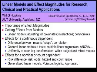
2. 100 d Chancesselected(%) c Activity b a 0 post r=0.57 Fitness Age pre strength Linear Models and Effect Magnitudes for Research, Clinical and Practical Applications • Importance of Effect Magnitudes • Getting Effects from Models • Linear models; adjusting for covariates; interactions; polynomials • Effects for a continuous dependent • Difference between means; “slope”; correlation • General linear models: t tests; multiple linear regression; ANOVA… • Uniformity of error; log transformation; within-subject and mixed models • Effects for a nominal or count dependent • Risk difference; risk, odds, hazard and count ratios • Generalized linear models: Poisson, logistic, log-hazard • Proportional-hazards regression Will G HopkinsAUT University, Auckland, NZ Sportscience 14, 49-57, 2010(sportsci.org/2010/wghlinmod)

3. Background: The Rise of Magnitude of Effects • Research is all about the effect of something on something else. • The somethings are variables, such as measures of physical activity, health, training, performance. • An effect is a relationship between the values of the variables, for example between physical activity and health. • We think of an effect as causal: more active  more healthy. • But it may be only an association: more active  more healthy. • Effects provide us with evidence for changing our lives. • The magnitude of an effect is important. • In clinical or practical settings: could the effect be harmful or beneficial? Is the benefit likely to be small, moderate, large…? • In research settings: • Effect magnitude determines sample size. • Meta-analysis is all about averaging magnitudes of study-effects. • So various research organizations now emphasize magnitude

4. Getting Effects from Models • An effect arises from a dependent variable and one or more predictor (independent) variables. • The relationship between the values of the variables is expressed as an equation or model. • Example of one predictor: Strength = a + b*Age • This has the same form as the equation of a line, Y = a + b*X, hence the term linear model. • The model is used as if it means: Strength  a + b*Age. • If Age is in years, the model implies that older subjects are stronger. • The magnitude comes from the “b” coefficient or parameter. • Real data won’t fit this model exactly, so what’s the point? • Well, it might fit quite well for children or old folks, and if so… • We can predict the average strength for a given age. • And we can assess how far off the trend a given individual falls.

5. Example of two predictors: Strength = a + b*Age + c*Size • Additional predictors are sometimes known as covariates. • This model implies that AgeandSize have effects on strength. • It’s still called a linear model (but it’s a plane in 3-D). • Linear models have an incredible property: they allow us to work out the “pure” effect of each predictor. • By pure here I mean the effect of Age on Strength for subjects of any given Size. • That is, what is the effect of Age if Size is held constant? • That is, yeah, kids get stronger as they get older, but is it just because they’re bigger, or does something else happen with age? • The something else is given by the “b”: if you hold Size constant and change Age by one year, Strength increases by exactly “b”. • We also refer to the effect of Age on Strengthadjusted forSize, controlled forSize, or (recently) conditioned onSize. • Likewise, “c” is the effect of one unit increase in Size for subjects of any given Age.

6. With kids, inclusion of Size would reduce the effect of Age. To that extent, Size is a mechanism or mediator of Age. • But sometimes a covariate is a confounder rather than a mediator. • Example: Physical Activity (predictor) has a strong relationship with Health (dependent) in elderly adults. Age is a confounder of the relationship, because Age causes bad health and inactivity. • Again, including potential confounders as covariates produces the pure effect of a predictor. • Think carefully when interpreting the effect of including a covariate: is the covariate a mechanism or a confounder? • If you are concerned that the effect of Age might differ for subjects of different Size, you can add an interaction… • Example of an interaction:Strength = a + b*Age + c*Size+ d*Age*Size • This model implies that the effect of Age on Strength changes with Size in some simple proportional manner (and vice versa). • It’s still known as a linear model.

7. You still use this model to adjust the effect of Age for the effect of Size, but the adjusted effect changes with different values of Size. • Another example of an interaction:Strength = a + b*Age + c*Age*Age = a + b*Age + c*Age2 • By interacting Age with itself, you get a non-linear effect of Age, here a quadratic. • If c turns out to be negative, this model implies strength rises to a maximum, then comes down again for older subjects. • To model something falling to a minimum, c would be positive. • To model more complex curvature, add d*Age3, e*Age4… • These are cubics, quartics…, but it’s rare to go above a quadratic. • These models are also known as polynomials. • They are all called linear models, even though they model curves. • Use the coefficients to get differences between chosen values of the predictor, and values of predictor and dependent at max or min. • Complex curvature needs non-linear modeling (see later) or linear modeling with the predictor converted to a nominal variable…

8. Group, factor, classification or nominal variables as predictors: • We have been treating Age as a number of years, but we could instead use AgeGroup, with several levels; e.g., child, adult, elderly. • Stats packages turn each level into a dummy variable with values of 0 and 1, then treat each as a numeric variable. Example: • Strength = a + b*AgeGroup is treated asStrength = a + b1*Child + b2*Adult + b3*Elderly, where Child=1 for children and 0 otherwise, Adult=1 for adults and 0 otherwise, and Elderly=1 for old folk and 0 otherwise. • The model estimates the mean value of the dependent for each level of the predictor: mean strength of children = a + b1. • And the difference in strength of adults and children is b2 – b1. • You don’t usually have to know about coding of dummies, but you do when using SPSS for some mixed models and controlled trials. • Dummy variables can also be very useful for advanced modeling. • For simple analyses of differences between group means with t‑tests, you don’t have to think about models at all!

9. Linear models for controlled trials • For a study of strength training without a control group:Strength = a + b*Trial, where Trial has values pre, post or whatever. • b*Trial is really b1*Pre + b2*Post, with Pre=1 or 0 and Post=1 or 0. • The effect of training on mean strength is given by b2 – b1. • For a study with a control group:Strength = a + b*Group*Trial, where Group has values expt, cont. • b*Group*Trial is reallyb1*ContPre+b2*ContPost+b3*ExptPre+b4*ExptPost. • The changes in the groups are given by b2 – b1 and b4 – b3. • The net effect of training is given by (b4 – b3) – (b2 – b1). • Stats packages also allow you to specify this model:Strength = a + b*Group + c*Trial + d*Group*Trial. • Group and Trial alone are known as main effects. • This model is really the same as the interaction-only model. • It does allow easy estimation of overall mean differences between groups and mean changes pre to post, but these are useless.

10. Or you can model change scores between pairs of trials. Example: • Strength = a + b*Group*Trial, where b has four values, is equivalent to StrengthChange = a + b*Group, where b has just two values (expt and cont) and StrengthChange is the post-pre change scores. • You can include subject characteristics as covariates to estimate the way they modify the effect of the treatment. Such modifiers or moderators account for individual responses to the treatment. • A popular modifier is the baseline (pre) score of the dependent:StrengthChange = a + b*Group + c*Group*StrengthPre. • Here the two values of c estimate the modifying effect of baseline strength on the change in strength in the two groups. • And c2 – c1 is the net modifying effect of baseline on the change. • Bonus: a baseline covariate improves precision of estimation when the dependent variable is noisy. • Modeling of change scores with a covariate is built into the controlled-trial spreadsheets at Sportscience.

11. You can include the change score of another variable as a covariate to estimate its role as a mediator (i.e., mechanism) of the treatment.Example: StrengthChange = a + b*Group + d*MediatorChange. • d represents how well the mediator explains the change in strength. • b2 – b1 is the effect of the treatment when MediatorChange=0;that is, the effect of the treatment not mediated by the mediator. • Linear vs non-linear models • Any dependent equal to a sum of predictors and/or their products is a linear model. • Anything else is non-linear, e.g., an exponential effect of Age, to model strength reaching a plateau rather than a maximum. • Almost all statistical analyses are based on linear models. • And they can be used to adjust for other effects, including estimation of individual responses and mechanisms. • Non-linear procedures are available but are more difficult to use.

12. Specific Linear Models, Effects and Threshold Magnitudes • These depend on the four kinds (or types) of variable. • Continuous (numbers with decimals): mass, distance, time, current; measures derived therefrom, such as force, concentration, volts. • Counts: such as number of injuries in a season. • Ordinal: values are levels with a sense of rank order, such as a 4-pt Likert scale for injury severity (none, mild, moderate, severe). • Nominal: values are levels representing names, such asinjured (no, yes), and type of sport (baseball, football, hockey). • As predictors, the first three can be simplified to numeric. • If a polynomial is inappropriate, parse into 2-5 levels of a nominal. • Example: Age becomes AgeGroup (5-14, 15-29, 30-59, 60-79, >79). • Values can also be parsed into equal quantiles (e.g., quintiles). • If an ordinal predictor such as a Likert scale has only 2-4 levels, or if the values are stacked at one end of the scale, analyze the values as levels of a nominal variable.

13. As dependents, each type of variable needs a different approach. • Continuous variables (e.g., time) and ordinals with enough levels (e.g., 7-pt Likert responses or their sums) need various forms of general linear model and general mixed linear model. • These models are unified by the assumption that the outcome statistic has a T sampling distribution. • Generalized linear models and generalized mixedlinear models are used with binary nominal variables coded into values of 0 or 1 (e.g., injured or not, rugby or not) and with counts coded as an integer (e.g., number of injuries). • These models take into account the special distributions of the dependent variable: binomial (for 0 and 1) and Poisson (for counts). • The general linear model is one of the generalized linear models. • Ordinal variables with only a few levels and nominals with several levels either need specific forms of generalized linear model or the levels can be grouped into a variable with values of only 0 and 1.

14. Dependent Predictor Effect of predictor Statistical model continuous nominal difference in means (un)paired t test; (multiple linear) reg-ression; ANOVA; ANCOVA Strength Trial continuous numeric "slope" (difference per unit of predictor); correlation Activity Age nominal count nominal nominal ratio of counts ratios of proportions, odds, rates, hazards InjuredNY Injuries Sex Sex count nominal numeric numeric "slope" (ratio per unit of predictor) "slope" (ratio per unit of predictor) SelectedNY Medals Fitness Cost • Effects and specific general linear models (with examples): • Effects and specific generalized linear models (with examples): logistic (log-odds), log-hazard, and proportional hazards (Cox) regressions Poisson regression

15. The most common effect statistic, for numberswith decimals (continuous variables). Difference when comparing different groups, e.g., patients vs healthy. Change when tracking the same subjects. Difference in the changes in controlled trials. The between-subject standard deviationprovides default thresholds for importantdifferences and changes. You think about the effect (mean) in terms of afraction or multiple of the SD (mean/SD). The effect is said to be standardized. The smallest important effect is ±0.20 (±0.20 of an SD). Strength Strength Trial patients healthy (means & SD) Strength pre post1 post2 Trial Dependent Predictor Effect continuous nominal difference or change in means

16. Trivial effect (0.1x SD) Very large effect (3.0x SD) post post pre pre Cohen Hopkins trivial <0.2 <0.2 small moderate 0.5-0.8 0.6-1.2 Complete scale: large >0.8 1.2-2.0 extremely large strength strength 0.2 0.6 1.2 2.0 4.0 trivial small moderate large very large ext. large very large ? ? 2.0-4.0 >4.0 • Example: the effect of a treatment on strength • Interpretation of standardizeddifference orchange in means: 0.2-0.5 0.2-0.6

17. area= 50% Standardized effect= 0.20 area= 58% athleteon 58th percentile Standardizedeffect Percentilechange strength 0.20 50  58 0.20 80  85 0.20 95  97 0.25 50  60 1.00 50  84 2.00 50  98 • Relationship of standardized effect to difference or change in percentile: athleteon 50th percentile strength • Can't define smallest effect for percentiles, because it depends what percentile you are on. • But it's a good practical measure. • And easy to generate with Excel, if the data are approx. normal.

18. Cautions with Standardizing • Choice of the SD can make a big difference to the effect. • Use the baseline (pre) SD, never the SD of change scores. • Standardizing works only when the SD comes from a sample representative of a well-defined population. • The resulting magnitude applies only to that population. • Beware of authors who show standard errors of the mean (SEM) rather than SD. • SEM = SD/(sample size) • So effects look a lot bigger than they really are. • Check the fine print; if authors have shown SEM, do some mental arithmetic to get the real effect. Other Smallest Differences or Changes in Means • Visual-analog scales scored as 0-10: 1 unit… • Single 5- to 7-pt Likert scales: half a step… • Athletic performance…

19. Visual-analog scales • The respondents indicate a perception on a line like this: Rate your pain by placing a mark on this scale: • Score the response as percent of the length of the line. • Magnitude thresholds: 10%, 30%, 50%, 70%, 90% for small, moderate, large, very large, extremely large differences or changes. • Likert scales • These are used for responses to questions like this: Over the last four weeks, how often did you train in a gym? not at allonce only2-3 timesonce a weektwice or more a week • Most Likert-type questions have four to seven choices. • Code them as integers (1, 2, 3, 4, 5…) and analyze as numerics. • Magnitude thresholds: consider the range as a visual analog scale; . • If you use the thresholds of the visual-analog scale as a guide, the threshold for a 6-pt scale would be ~0.5, 1.5, 2.5, 3.5 and 4.5.   none unbearable

20. 0.3 0.9 1.6 2.5 4.0 trivial small moderate large very large ext. large Measures of Athletic Performance • For fitness tests of team-sportathletes, use standardization. • For top solo athletes, an enhancement that results in one extra medal per 10 competitions is the smallest important effect. • Simulations show this enhancement is achieved with 0.3 of an athlete's typical variability from competition to competition. • Example: if the variability is a coefficient of variation of 1%, the smallest important enhancement is 0.3%. • Note that in many publications I have mistakenly referred to 0.5 of the variability as the smallest effect. • Moderate, large, very large and extremely large effects result in an extra 3, 5, 7 and 9 medals in every 10 competitions. • The corresponding enhancements as factors of the variability are:

21. Beware: smallest effect on athletic performance in performance tests depends on method of measurement, because… • A percent change in an athlete's ability to output power results in different percent changes in performance in different tests. • These differences are due to the power-duration relationship for performance and the power-speed relationship for different modes of exercise. • Example: a 1% change in endurance power output produces the following changes… • 1% in running time-trial speed or time; • ~0.4% in road-cycling time-trial time; • 0.3% in rowing-ergometer time-trial time; • ~15% in time to exhaustion in a constant-power test. • A hard-to-interpret change in any test following a fatiguing pre-load. (But such tests can be interpreted for cycling road races: see Bonetti and Hopkins, Sportscience 14, 63-70, 2010.)

22. Activity Age Activity Age 0.1 0.3 0.5 0.7 0.9 trivial small moderate large very large ext. large Dependent Predictor Effect continuous numeric "slope" (difference per unit of predictor); correlation • A slope is more practical than a correlation. • But unit of predictor is arbitrary, so it'shard to define smallest effect for a slope. • Example: -2% per year may seem trivial,yet -20% per decade may seem large. • For consistency with interpretation of correlation, better to express slope as difference per two SDs of predictor. • It gives the difference between a typically low and high subject. • See the page on effect magnitudes at newstats.org for more. • Easier to interpret the correlation, using Cohen's scale. • Smallest important correlation is ±0.1. Complete scale: • But note: in validity studies, correlations >0.90 are desirable. r=-0.57

23. The effect of a nominal predictor can also be expressed as a correlation = √(fraction of “variance explained”). • A 2-level predictor scored as 0 and 1 gives the same correlation. • With equal number of subjects in each group, the scales for correlation and standardized difference match up. • For >2 levels, the correlation can’t be applied to individuals. Avoid. • Correlations when controlling for something… • Interpreting slopes and differences in means is no great problem when you have other predictors in the model. • Be careful about which SD you use to standardize. • But correlations are a challenge. • The correlation is either partial or semi-partial (SPSS: "part"). • Partial = effect of the predictor within a virtual subgroup of subjects who all have the same values of the other predictors. • Semi-partial = unique effect of the predictor with all subjects. • Partial is probably more appropriate for the individual. • Confidence limits may be a problem in some stats packages.

24. The Names of Linear Models with a Continuous Dependent • You need to know the jargon so you can use the right procedure in a spreadsheet or stats package. • Unpaired t test: for 2 levels of a single nominal predictor. • Use the unequal-variances version, never the equal-variances. • Paired t test: as above, but the 2 levels are for the same subjects. • Simple linear regression: a single numeric predictor. • Multiple linear regression: 2 or more numeric predictors. • Analysis of variance (ANOVA): one or more nominal predictors. • Analysis of covariance (ANCOVA): one or more nominal and one or more numeric predictors. • Repeated-measures analysis of (co)variance: AN(C)OVA in which each subject has two or more measurements. • General linear model (GLM): any combination of predictors. • In SPSS, nominal predictors are factors, numerics are covariates. • Mixed linear model: any combination of predictors and errors.

25. The Error Term in Linear Models with a Continuous Dependent • Strength = a + b*Age isn’t quite right for real data, becauseno subject’s data fit this equation exactly. • What’s missing is a different error for each subject:Strength = a + b*Age + error • This error is given an overall mean of zero, and it varies randomly (positive and negative) from subject to subject. • It’s called the residual error, and the values are the residuals. • residual = (observed value) minus (predicted value) • In many analyses the error is assumed to have values that come from a normal (bell-shaped) distribution. • This assumption can be violated. Testing for normality is silly. The Central Limit Theorem assures a normal sampling distribution. • With a count as the dependent, the error has a Poisson distribution, which is an issue • Address with generalized linear modeling–see later.

26. You characterize the error with a standard deviation. • It’s also known as the standard error of the estimate or the root mean square error. • In general linear models, the error is assumed to be uniform. • That is, there is only one SD for the residuals, or the error for every datum is drawn from a single “hat”. • Non-uniform error is known as heteroscedasticity. • If you don’t do something about it, you get wrong answers. • Without special treatment, many datasets show bigger errors for bigger values of the dependent. • This problem is obvious in some tables of means and SDs, in scatter plots, or in plots of residual vs predicted values (see later). • Such plots of individual values are also good for spotting outliers. • It arises from the fact that effects and errors in the data are percents or factors, not absolute values. • Example: an error or effect of 5% is 5 s in 100 s but 10 s in 200 s.

27. Address the problem by analyzing the log-transformed dependent. • 5% effect means Post = Pre*1.05. • Therefore log(Post) = log(Pre) + log(1.05). • That is, the effect is the same for everyone: log(1.05). • And we now have a linear (additive) model, not a non-linear model, so we can use all our usual linear modeling procedures. • A 5% error means typically 1.05 and 1.05, or 1.05. • And a 100% error means typically 2.0 (i.e., values vary typically by a factor of 2), and so on. • When you finish analyzing the log-transformed dependent, you back-transform to a percent or factor effect using exponential e. • Show percents for anything up to ~30%. Show factors otherwise, e.g., when the dependent is a hormone concentration. • Use the log-transformed values when standardizing. • Log transformation is often appropriate for a numeric predictor. • The effect of the predictor is then expressed per percent, per 10%, per 2-fold increase, and so on.

28. Dependent 100*ln(Dependent) 1000 6000 Residual 800 4000 Predicted 600 2000 400 Dependent (log scale) 0 10000 200 0 -2000 1000 3 4 5 6 7 8 9 3 4 5 6 7 8 9 Predictor Predictor 100 Residuals Residuals 10 3000 100 1 2000 3 4 5 6 7 8 9 50 Predictor 1000 0 0 Non-uniform scatter -50 -1000 Uniform scatter -2000 -100 0 2000 4000 250 500 750 1000 Predicteds Predicteds • Example of simple linear regression with a dependent requiring log transformation. • A log scale or log transformation produces uniform residuals.

29. Rank transformation for non-normality and non-uniformity? • Sort all the values of the dependent variable, rank them (i.e., number them 1, 2, 3,…), then use this rank in all further analyses. • The resulting analyses are sometimes called non-parametric. • But it’s still linear modeling, so it’s really parametric. • They have names like Wilcoxon and Kruskal-Wallis. • Some are truly non-parametric: the sign test; neural-net modeling. • Some researchers think you have to use this approach when “the data are not normally distributed”. • In fact, the rank-transformed dependent is anything but normally distributed: it has a uniform (flat) distribution!!! • Does rank transformation deal with uniformity of effects and error? • No! Example: with 100 observations, there is no way the difference between rank 1 and 2 is the same effect as the difference between 50 and 51 (or 99 and 100, for athletic performance). • So NEVER use raw rank transformation. • But log(rank) appears to work well for athletic performance.

30. Non-uniformity also arises with different groups and time points. • Example: a simple comparison of means of males and females, with different SD for males and females (even after log transformation). • Hence the unequal-variances t statistic or test. • To include covariates here, you can’t use the general linear model: you have to keep the groups separate, as in my spreadsheets. • Example: a controlled trial, with different errors at different time points arising from individual responses and changes with time. • MANOVA and repeated-measures ANOVA can give wrong answers. • Address by reducing or combining repeated measurements into a single change score for each subject: within-subject modeling. • Then allow for different SD of change scores by analyzing the groups separately, as above. • Bonus: you can calculate individual responses as an SD. • See Repeated Measures and Random Effects at sportsci.org and/or the article on the controlled-trial spreadsheets for more. • Or specify several errors and much more with a mixed model...

31. Mixed modeling is the cutting-edge approach to the error term. • Mixed = fixed effects + random effects. • Fixed effects are the usual terms in the model; they estimate means. • Fixed, because they have the same value for everyone in a group or subgroup; they are not sampled randomly. • Random effects are error terms and anything else randomly chosen from some population; each is summarized with an SD. • The general linear model allows only one error. Mixed models allow: • specification of different errors between and within subjects; • within-subject covariates (GLM allows only subject characteristics or other covariates that do not change between trials); • specification of individual responses to treatments and individual differences in subjects’ trends; • interdependence of errors and other random effects, which arises when you model different lines or curves for each subject. • With repeated measurement in controlled trials, simplify analyses by analyzing change scores, even when using mixed modeling.

32. InjuredNY Sex Dependent Predictor Effect nominal nominal difference of proportions; ratios of proportions, odds, rates, hazards, mean event time • Example: a dependent scored as 0 or 1 (injured no or yes) predicted by sex (female, male) of playersin a season of touch rugby. • Convert the 0s and 1s in each group to proportions by averaging, then multiplyby 100 to express as percents. • Risk difference or proportion difference • A common measure. Example: a-b = 75%-36% = 39%. • Problem: the sense of magnitude of a given difference depends on how big the proportions are. • Example: for a 10% difference, 90% vs 80% doesn't seem big, but… 11% vs 1% can be interpreted as a huge "difference" (11x the risk). 100 Proportioninjured (%) a =75% b =36% 0 male female Sex

33. 1.0 3.0 5.0 7.0 9.0 trivial small moderate large very large ext. large 100 Proportioninjured (%) a =75% • So there is no scale of magnitudes for a risk or proportion difference. • Exception: effects on winning a close match can be expressed as a proportion difference: 55% vs 45% is a 10% difference or 1 extra match in every 10 matches; 65% vs 35% is 3 extra, and so on. • Hence this scale for extra matches won or lost per 10 matches: • But the analyses (models) don't work properly with proportions. • We have to use odds or hazards instead of proportions. Stay tuned. • Risk ratio (relative risk) or proportion ratio • Another common measure.Example: a/b = 75/36 = 2.1, which means males are "2.1 times more likely" to be injured,or "a 110% increase in risk" of injury for males. b =36% 0 male female Sex

34. 1.11 1.43 2.0 3.3 10 trivial small moderate large very large ext. large • Problem: if it's a time dependent measure, and youwait long enough, everyone gets affected, so risk ratio = 1.00. • But it works for rare time-dependent risks and for time-independent classifications (e.g., proportion playing a sport). • Smallest important effect:for every 10 injured males there are 9 injured females. • That is, one in 10 injuries is due to being male. • If there are N males and N females, risk ratio = (10/N)/(9/N) = 10/9. • Similarly, moderate, large, very large and extremely large effects:for every 10 injured males, there are 7, 5, 3 and 1 injured females. • Corresponding risk ratios are 10/7, 10/5, 10/3 and 10/1. • Hence this complete scale for proportion ratio and low-risk ratio: • and the inverses for reductions in proportions: 0.9, 0.7, 0.5, 0.3, 0.1. • But still no way to model proportions, especially to get ratio effects. • Two solutions: hazards instead of risks; odds instead of proportions.

35. Hazard ratio for time-dependent events. • To understand hazards, considerthe increase in proportions with time. • Over a very short period, the riskin both groups is tiny, and the risk ratiois independent of time. • Example: risk for females = a = 0.28% per 1 d = 0.56% per 2 d, risk for males = b = 0.11% per 1 d = 0.22% per 2d. So risk ratio = a/b = 0.28/0.11 = 0.56/0.22 = 2.5. That is, females are 2.5x more likely to get injuredper unit time, whatever the (small) unit of time. • The risk per unit time is called a hazard or incidence rate. • Hence hazard ratio, incidence-rate ratio or “right-now” risk ratio. • It can also be interpreted as the ratio of the times taken for the same proportion to get affected in two groups. • Example: males take 2.5x as long to get injured as females. 100 females Proportioninjured (%) males 0 Time (months) a b

36. a b 1.11 1.43 2.0 3.3 10 trivial small moderate large very large ext. large 100 males • By the time lots of males or females are injured, the observed risk ratio drops below the hazard ratio. • Example: at 5 weeks, the hazard ratio may still be 2.5, but the risk ratio = a/b = 75/36 = 2.1. • The hazard ratio for those still uninjuredis usually assumed to stay the same, even if the hazards change with time. • Example: the risk of injury might increase laterin the season for both sexes, but the risk ratio for new injuries(the hazard ratio) doesn't change. A big plus! • And hazards and hazard ratios can be modeled! • Magnitude thresholds must be the same as for the risk ratio, even for frequent events, because such events start off rare. • Hence this scale for the hazard ratio: • and the inverses 0.9, 0.7, 0.5, 0.3, 0.1. Proportioninjured(%) females 0 Time (months)

37. 100 c =25% d =64% Proportionplaying(%) a =75% • Odds ratio for time-independent classifications. • Odds are the awkward but only way to model classifications. • Example: proportion of kids playing sport. • Odds of a male playing = a/c = 75/25. • Odds of a female playing = b/d = 36/64. • Odds ratio = (75/25)/(36/64) = 5.3. • Interpret the ratio as "…times more likely" onlywhen the proportions in both groups are small (<10%). • The odds ratio is then approximately equal to the proportion ratio. • Magnitude thresholds have to be converted from the values for the proportion ratio, using the proportion in the reference group. • Example: with females = 36%, proportion of males corresponding to the smallest proportion of 10/9 is (10/9)*36 = 40%, so the odds ratio for the smallest increase = (40/60)/(36/64) = 1.19. • And proportion of males for smallest decrease is (9/10)*36 = 32.4%, so odds ratio for the smallest decrease = (32.4/67.6)/(36/64) = 0.85. • Note that 1.19 and 0.85 are not the inverse of each other. b =36% 0 male female Sex

38. Odds ratio in case-control studies • In these studies, the outcome is the odds for the "exposure" in cases divided by the odds for the exposure in controls. • If the controls are sampled as the cases come in ("incidence density sampling", the proper approach), this odds ratio is equivalent to the hazard ratio for incidence of cases in exposed and unexposed groups (the usual prospective cohort study). • So you can interpret the odds ratio in the usual way as "times as likely" to be affected if you are exposed. • If the controls are sampled in one go after the cases have accumulated, the odds ratio has to be converted to a hazard ratio. • Similarly if the cases are time-independent classifications (e.g., cases = Olympians, controls = non-Olympian athletes), the odds ratio of exposure (e.g., family member an Olympian) has to be converted to a risk ratio before it represents "times as likely" that the exposure will produce the classification.

39. Relationships between risk, hazard and odds ratios • Given odds = p/(1-p), where p = proportion (as a fraction, not %), it follows that p = odds/(1+odds). • You can use algebra to convert between an odds ratio and a risk or proportion ratio, but you need the proportion in the reference group. • Example: odds ratio = OR = [p2/(1-p2)]/[p1/(1-p1)], • Therefore risk ratio = RR = p2/p1 = OR/[1+p1(OR-1)]. • This formula allows you to convert modeledodds ratios and confidence limits into risk ratios and risk differences, at a given value of proportion in the reference group. • Conversions to hazard ratios dependon assuming constant hazards. • In a small interval dt, dp = (1-p).h.dt,where h is the hazard (probability per unit time). • Hence p=(1-e-h.t), and p2/p1=(1-e-h2.t)/(1-e-h1.t). • Can show that risk ratio < hazard ratio < odds ratio. • And if p1 and p2 are <10%, all three are approximately equal. 1 p2=1-e-h2.t Probability(p) p1=1-e-h1.t 0 Time

40. 100 males Proportioninjured (%) t1 t2 females 0 Time • Ratio of mean time to event = t2/t1. • If the hazards are constant, t2/t1 isthe inverse of the hazard ratio. • Example: if hazard ratio is 2.5, there is 2.5x the risk of injury. But 1/2.5 = 0.40,so the same proportion of injuries occursin 0.40 (less than half) of the time, on average. • Number needed to treat (NNT) = 100/(risk difference (%)). • The number you would have to treat or sample for one subject to have an outcome attributable to the effect. • Promoted in some clinical journals, but not widely used. • Can’t estimate directly with linear models. • Problems with its confidence limits. Other Magnitude Scales for Proportions and Risks • I haven’t found any. • The first version of this article had different magnitude scales for odds ratios with common classifications and hazard ratios with common events.

41. SelectedNY Fitness Dependent Predictor Effect nominal numeric "slope" (difference or ratio per unit of predictor) • Derive and interpret the “slope” (a correlation isn’t defined here). • As with a nominal predictor, you have to estimate effects as odds ratios (for time-independent classifications)or hazard ratios (for time-dependent events)to get confidence limits. • Example shows individual values, the way the modeled chances would change with fitness, and the meaning of the odds ratio per unit of fitness: (b/d)/(a/c). • Odds ratio here is ~ (75/25)/(25/75) = 9.0 per unit of fitness. • Best to express as odds or hazard ratio per 2 SD of predictor. 100 d Chancesselected(%) c b a 0 Fitness

42. 1.11 1.43 2.0 3.3 10 trivial small moderate large very large ext. large Dependent Predictor Effect count nominal ratio of counts Injuries Sex • Effect of a nominal predictor is expressed as a ratio (factor) or percent difference. • Example: in their sporting careers, women get 2.3 times more tendon injuries than men. • Example: men get 26% (1.26x) more muscle sprains than women. • Effects of a numeric predictor are expressed as factors or percents per unit or per 2 SD of the predictor. • Example: 13% more tackles per 2 SD of repeated-sprint speed. • Magnitude scale for the count ratio is the same as for proportion and hazard ratios (and their inverses): count numeric "slope" (ratio per unit of predictor) Tackles Fitness

43. Details of Linear Models for Events, Classifications, Counts • Counts, and binary variables representing levels of a nominal give wrong answers as dependents in the general linear model. • It can predict negative or non-integral values, which are impossible. • Non-uniformity would also be an issue. • Generalized linear modeling has been devised for such variables. • The generalized linear model predicts a dependent that can range continuously from ‑ to +, just as in the general linear model. • You specify the dependent by specifying the distribution of the dependent and a link function. • For a continuous dependent, specifying the normal distribution and the identity link produces the general linear model. • Don’t use this approach with continuous dependents, because the standard procedures for general linear modeling are easier. • Easiest to understand the approach with counts first…

44. For counts (e.g., each athlete’s number of injuries), the dependent is the log of the mean count. • The mean count ranges continuously from 0 to +. • The log of the mean count ranges from - to +. • So the link function is the log. • Specify the distribution for counts, Poisson. • The model is called Poisson regression. • The log link results in effects expressed as count ratios. • If the counts accumulate over different periods for different subjects, you can specify the period in the model as an offset or denominator. • You are then modeling rates, and the effects are rate ratios. • With advanced stats packages you can include an over-dispersionfactor to allow for data that don't fit a Poisson distribution properly (or a binomial distribution, when the dependent is a proportion). • For example, the counts for each subject tend to occur in clusters. • The model thereby reflects the fact that the counts have a bigger variation for a given predicted count than purely Poisson counts.

45. For binary variables representing time-independent events(e.g., selected or not), the dependent is the log of the odds of the event occurring. • Odds=p/(1-p), where p is the probability of the event. • P ranges from 0 to 1, so odds range continuously from 0 to +. • So log of the odds ranges from - to +. • So the link function is the log-odds, also known as the logit. • Specify the distribution for binary events, binomial. • The model is called logistic regression, but log-odds regression would be better. • The log of the odds results in effects expressed as odds ratios. • A log-odds model may be simplistic or unrealistic, but it’s got to be better than modeling p or log p, which definitely does not work. • Some researchers mistakenly use this model for time-dependent events, such as development of injury. But… • If proportions of subjects experiencing the event are low, you can model risk, odds or hazards, because the ratios are the same.

46. For binary variables representing time-dependent events(e.g., un/injured), the dependent is the log of the hazard. • The hazard is the probability of the event per unit time. • For events that accumulate with a constant hazard (h), the proportion of subjects affected at time t is given via calculus by p = 1 - e-h.t; hence h = hazard = -log(1 - p). • The hazard ranges continuously from 0 to +. • Log of the hazard ranges from - to +. • The link function is known confusingly as the complementary log-log: log(-log(1-p)). • I prefer to refer to the log-hazard link. • Specify the distribution for binary events, binomial. • The model has no common name. I call it log-hazard regression. • The log of the hazard results in effects expressed as hazard ratios. • You can specify a different monitoring time for each subject. • When hazards aren’t constant, use proportional hazards regression.

47. Dependent Effect of predictor Statistical model multiple proportionschoice of several sports odds ratio multinomial logistic regression ordinalinjury severity (4-pt Likert) odds or hazard ratio cumulative logistic or hazard regression time to eventtime to injury hazard ratio proportional-hazards (Cox) regression The next three slides are for experts.Other Models for Classifications and Events • There are several other more complex models. • All have outcomes modeled as ratios (between levels of nominal predictors) or ratios per unit (or per 2 SD) of numeric predictors. • The magnitude scales are the same as in the simpler models. • Summary (with examples):

48. When the dependent is a nominal with >2 levels, group into various combinations of 2 levels and use simpler models, or… • Multinomial logistic regression, for time-independent nominals(e.g., a study of predictors of choice of sport). • Use the multinomial distribution and the generalized logit link (available in SAS in the Glimmix procedure). • SAS does not provide a link in Glimmix or Genmod for multinomial hazard regression of time-dependent nominals. • Cumulative logistic regression, for time-independent ordinals (e.g.: lose, draw, win a game; injury severity on a 4-point Likert scale). • Multinomial distribution; cumulative logit link. • Use for <5-pt or skewed Likert scales; otherwise use general linear. • Cumulative hazard regression, for time-dependent ordinals(e.g., uninjured, mild injury, moderate injury, severe injury). • Multinomial distribution; cumulative complementary log-log link. • Generalized linear models for repeated or clustered measures are also known as generalized estimating equations.

49. Proportioninjured (%) 100 males females 0 Time (months) • Proportional hazards (Cox) regression is another and more advanced form of linear modeling for time-dependent events. • Use when hazards can change with time,if you can assume ratios of thehazards of the effects are constant. • Example: hazard changes as the season progresses, but hazard for malesis always 1.5x that for females. • A constant ratio is not obvious in this kind of figure. • Time to the event is the dependent, but effects are estimated and interpreted as hazard ratios. • The model takes account of censoring: when someone leaves the study (or the study stops) before the event has occurred. • Not covered in this presentation: magnitude thresholds for measures of reliability, validity, and diagnostic accuracy.

50. Main Points • An effect is a relationship between a dependent and predictor. • Effect magnitudes have key roles in research and practice. • Magnitudes are provided by linear models, which allow for adjustment, interactions, and polynomial curvature. • Continuous dependents need various general linear models. • Examples: t tests, multiple linear regression, ANOVA… • Within-subject and mixed modeling allow for non-uniformity of error arising from different errors with different groups or time points. • Effects for continuous dependents are mean differences, slopes (expressed as 2 SD of the predictor), and correlations. • Thresholds for small, moderate, large, very large and extremely large standardized mean differences: 0.20, 0.60, 1.2, 2.0, 4.0. • Thresholds for correlations: 0.10, 0.30, 0.50, 0.70, 0.90. • Many dependent variables need log transformation before analysis to express effects and errors as uniform percents or factors.