Inference for Regression: Understanding Population and Sample Relationships
550 likes | 671 Views
In this lesson, we explore regression inference by fitting a regression line to a sample of 59 observations from Nambe Mills. We analyze the population mean relationship between the variables, considering the variability of y-values and the assumptions required for reliable inference. These assumptions include linearity, independence, equal variance, and normal population distribution. Additionally, we discuss how to test the null hypothesis for the regression slope, interpreting the significance of the results and understanding the standard error of the slope.

Inference for Regression: Understanding Population and Sample Relationships
E N D
Presentation Transcript
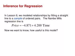
Inference for Regression • In Lesson 6, we modeled relationships by fitting a straight line to a sample of ordered pairs. The Nambe Mills regression line is • Now we want to know, how useful is this model?
16.1 The Population and the Sample The Nambe Mills sample is based on 59 observations. But we know observations vary from sample to sample. So we imagine a true line that summarizes the relationship between x and y for the entire population, Where µy is the population mean of y at a given value of x. We write µy instead of y because the regression line assumes that the means of the y values for each value of x fall exactly on the line.
16.1 The Population and the Sample • For a given value x: • Most, if not all, of the y values obtained from a particular sample will not lie on the line. • The sampled y values will be distributed aboutµy. • We can account for the difference between ŷ and µy by adding the error residual, or ε:
16.1 The Population and the Sample • Regression Inference • Collect a sample and estimate the population β’s by finding a regression line (Chapter 6): • The residuals e = y – ŷ are the sample based versions of ε. • Account for the uncertainties in β0 and β1 by making confidence intervals, as we’ve done for means and proportions.
16.2 Assumptions and Conditions • The inference methods of Chapter 16 are based on these assumptions (check these assumptions in this order): • Linearity Assumption • Independence Assumption • Equal Variance Assumption • Normal Population Assumption
16.2 Assumptions and Conditions The inference methods of Chapter 16 are based on these assumptions (check these assumptions in this order): Linearity Assumption – This condition is satisfied if the scatterplot of x and y looks straight. 2. Independence Assumption –Look for randomization in the sample or the experiment. Also check the residual plot for lack of patterns.
16.2 Assumptions and Conditions 3. Equal Variance Assumption – Check the Equal Spread Condition, which means the variability of y should be about the same for all values of x. 4. Normal Population Assumption – Assume the errors around the idealized regression line at each value of x follow a Normal model. Check if the residuals satisfy the Nearly Normal Condition.
16.2 Assumptions and Conditions Summary of Assumptions and Conditions
16.2 Assumptions and Conditions Summary of Assumptions and Conditions • Make a scatterplot of the data to check for linearity. (Linearity Assumption) • Fit a regression and find the residuals, e, and predicted values ŷ. • Plot the residuals against time (if appropriate) and check for evidence of patterns (Independence Assumption). • Make a scatterplot of the residuals against x or the predicted values. This plot should not exhibit a “fan” or “cone” shape. (Equal Variance Assumption)
16.2 Assumptions and Conditions Testing the Assumptions, continued 5. Make a histogram and Normal probability plot of the residuals (Normal Population Assumption) Data from Nambé Mills (Chapter 8)
16.3 The Standard Error of the Slope For a sample, we expect b1 to be close, but not equal to the model slope β1. For similar samples, the standard error of the slope is a measure of the variability of b1 about the true slope β1.
16.3 The Standard Error of the Slope Which of these scatterplots would give the more consistent regression slope estimate if we were to sample repeatedly from the underlying population? Hint: Compare se’s.
16.3 The Standard Error of the Slope Which of these scatterplots would give the more consistent regression slope estimate if we were to sample repeatedly from the underlying population? Hint: Compare sx’s.
16.3 The Standard Error of the Slope Which of these scatterplots would give the more consistent regression slope estimate if we were to sample repeatedly from the underlying population? Hint: Compare n’s.
16.4 A Test for the Regression Slope The usual null hypothesis about the slope is that it’s equal to 0. Why? A slope of zero says that y doesn’t tend to change linearly when x changes. In other words, if the slope equals zero, there is no linear association between the two variables.
16.4 A Test for the Regression Slope • Example : Soap • A soap manufacturer tested a standard bar of soap to see how long it would last. A test subject showered with the soap each day for 15 days and recorded the weight (in grams) remaining. Conditions were met so a linear regression gave the following: • Dependent variable is: Weight • R squared = 99.5% s = 2.949 • Variable Coefficient SE(Coeff) t-ratio P-value • Intercept 123.141 1.382 89.1 <0.0001 • Day -5.57476 0.1068 -52.2 <0.0001 • What is the standard deviation of the residuals? • What is the standard error of ? • What are the hypotheses for the regression slope? • At α = 0.05, what is the conclusion?
16.4 A Test for the Regression Slope • Example : Soap • A soap manufacturer tested a standard bar of soap to see how long it would last. A test subject showered with the soap each day for 15 days and recorded the weight (in grams) remaining. Conditions were met so a linear regression gave the following: • Dependent variable is: Weight • R squared = 99.5% s = 2.949 • Variable Coefficient SE(Coeff) t-ratio P-value • Intercept 123.141 1.382 89.1 <0.0001 • Day -5.57476 0.1068 -52.2 <0.0001 • What is the standard deviation of the residuals? se= 2.949What is the standard error of ? SE( ) = 0.0168
16.4 A Test for the Regression Slope • Example : Soap • A soap manufacturer tested a standard bar of soap to see how long it would last. A test subject showered with the soap each day for 15 days and recorded the weight (in grams) remaining. Conditions were met so a linear regression gave the following: • Dependent variable is: Weight • R squared = 99.5% s = 2.949 • Variable Coefficient SE(Coeff) t-ratio P-value • Intercept 123.141 1.382 89.1 <0.0001 • Day -5.57476 0.1068 -52.2 <0.0001 • What are the hypotheses for the • regression slope? • At α = 0.05, what is the conclusion? Since the p-value is small (<0.0001), reject the null hypothesis. There is strong evidence of a linear relationship between Weight and Day.
16.4 A Test for the Regression Slope • Example : Soap • A soap manufacturer tested a standard bar of soap to see how long it would last. A test subject showered with the soap each day for 15 days and recorded the weight (in grams) remaining. Conditions were met so a linear regression gave the following: • Dependent variable is: Weight • R squared = 99.5% s = 2.949 • Variable Coefficient SE(Coeff) t-ratio P-value • Intercept 123.141 1.382 89.1 <0.0001 • Day -5.57476 0.1068 -52.2 <0.0001 • Find a 95% confidence interval for the slope? • Interpret the 95% confidence interval for the slope? • At α = 0.05, is the confidence interval consistent with the hypothesis test conclusion?
16.4 A Test for the Regression Slope • Example : SoapA soap manufacturer tested a standard bar of soap to see how long it would last. A test subject showered with the soap each day for 15 days and recorded the weight (in grams) remaining. Conditions were met so a linear regression gave the following: • Dependent variable is: Weight • R squared = 99.5% s = 2.949 • Variable Coefficient SE(Coeff) t-ratio P-value • Intercept 123.141 1.382 89.1 <0.0001 • Day -5.57476 0.1068 -52.2 <0.0001 • Find a 95% confidence interval for the slope? • Interpret the 95% confidence interval for the slope? We can be 95% confident that weight of soap decreases by between 5.34 and 5.8 grams per day. • At α = 0.05, is the confidence interval consistent with the hypothesis test conclusion? Yes, the interval does not contain zero, so reject the null hypothesis.
16.5 A Hypothesis Test for Correlation What if we want to test whether the correlation between x and y is 0?
16.6 Standard Errors for Predicted Values SE becomes larger the further xν gets from . That is, the confidence interval broadens as you move away from . (See figure at right.)
16.6 Standard Errors for Predicted Values SE, and the confidence interval, becomes smaller with increasing n. SE, and the confidence interval, are larger for samples with more spread around the line (when se is larger).
16.6 Standard Errors for Predicted Values Because of the extra term , the confidence interval for individual values is broader that those for the predicted mean value.
16.7 Using Confidence and Prediction Intervals Confidence interval for a mean: The result at 95% means “We are 95% confident that the mean value of y is between 4.40 and 4.70 when x= 10.1.”
16.7 Using Confidence and Prediction Intervals Prediction interval for an individual value: The result at 95% means “We are 95% confident that a single measurement of y will be between 3.95 and 5.15 when x= 10.1.”
16.7 Using Confidence and Prediction Intervals Example : External Hard Disks A study of external disk drives reveals a linear relationship between the Capacity (in GB) and the Price (in $). Regression resulted in the following: Find the predicted Price of a 1000 GB hard drive. Find the 95% confidence interval for the mean Price of all 1000 GB hard drives. Find the 95% prediction interval for the Price of one 1000 GB hard drive.
16.7 Using Confidence and Prediction Intervals Example : External Hard Disks A study of external disk drives reveals a linear relationship between the Capacity (in GB) and the Price (in $). Regression resulted in the following: Find the predicted Price of a 1000 GB hard drive.
16.7 Using Confidence and Prediction Intervals Example : External Hard Disks A study of external disk drives reveals a linear relationship between the Capacity (in GB) and the Price (in $). Regression resulted in the following: Find the 95% confidence interval for the mean Price of all 1000 GB hard drives.
16.7 Using Confidence and Prediction Intervals Example : External Hard Disks A study of external disk drives reveals a linear relationship between the Capacity (in GB) and the Price (in $). Regression resulted in the following: Find the 95% prediction interval for the Price of one 1000 GB hard drive.
Don’t fit a linear regression to data that aren’t straight. • Watch out for changing spread. • Watch out for non-Normal errors. Check the histogram and the Normal probability plot. • Watch out for extrapolation. It is always dangerous to predict for x-values that lie far away from the center of the data.
Watch out for high-influence points and unusual observations. • Watch out for one-tailed tests. Most software packages perform only two-tailed tests. Adjust your P-values accordingly.
What Have We Learned? • Apply your understanding of inference for means using Student’s t to inference about regression coefficients. • Know the Assumptions and Conditions for inference about regression coefficients and how to check them, in this order: • Linearity • Independence • Equal Variance • Normality
What Have We Learned? • Know the components of the standard error of the slope coefficient: • The standard deviation of the residuals, • The standard deviation of x, • The sample size, n
What Have We Learned? • Be able to find and interpret the standard error of the slope. • The standard deviation of the residuals, • The standard error of the slope is the estimated standard deviation of the sampling distribution of the slope.
What Have We Learned? • State and test the standard null hypothesis on the slope. • H0: β1 = 0. This would mean that x and y are not linearly related. • We test this null hypothesis using the t-statistic
What Have We Learned? • Know how to use a t-test to test whether the true correlation is zero. • Construct and interpret a confidence interval for the predicted mean value corresponding to a specified value, xn. where
What Have We Learned? • Construct and interpret a confidence interval for an individual predicted value corresponding to a specified value, xn. where
17.1 Examining Residuals for Groups Consider the following study of the Sugar content vs. the Calorie content of breakfast cereals: There is no obvious departure from the linearity assumption.
17.1 Examining Residuals for Groups The histogram of residuals looks fairly normal…
17.1 Examining Residuals for Groups …but the distribution shows signs of being a composite of three groups of cereal types. The mean Calorie content may depend on some factor besides sugar content.
17.1 Examining Residuals for Groups Examining the residuals of groups… …suggests factors other than sugar content that may be important in determining Calorie content. Puffing: replacing cereal with “air” lowers the Calorie content, even for high-sugar cereals Fat/oil: Fats add to the Calorie content, even for low-sugar cereals Puffed cereals (high air content per serving) Cereals with fruits and/or nuts (high fat/oil content per serving) All others
17.1 Examining Residuals for Groups Conclusion: It may be better to report three regressions, one for puffed cereals, one for high-fat cereals, and one for all others.
17.1 Examining Residuals for Groups Example : Concert Venues A concert production company examined it’s records and made the following scatterplot. The company places concerts in two venues, a smaller, more intimate theatre (plotted with blue circles) and a larger auditorium style venue. Describe the relationship between Talent Cost and Total Revenue. How are the results for the two venues similar? Different?
17.1 Examining Residuals for Groups Example : Concert Venues A concert production company examined it’s records and made the following scatterplot. The company places concerts in two venues, a smaller, more intimate theatre (plotted with blue circles) and a larger auditorium style venue. Describe the relationship between Talent Cost and Total Revenue. Positive, linear, and moderately strong. As Talent Cost increases, Revenue also increases.
17.1 Examining Residuals for Groups Example : Concert Venues A concert production company examined it’s records and made the following scatterplot. The company places concerts in two venues, a smaller, more intimate theatre (plotted with blue circles) and a larger auditorium style venue. How are the results for the two venues similar? Both venues show an increase of revenue with talent cost. Different? The larger venue has greater variability. Revenue for that venue is more difficult to predict.
17.1 Examining Residuals for Groups Example : Concert Venues A concert production company examined it’s records and made the following scatterplot. The company places concerts in two venues, a smaller, more intimate theatre (plotted with blue circles) and a larger auditorium style venue. How are the results for the two venues different? The larger venue has greater variability. Revenue for that venue is more difficult to predict.
