Chapter 15 Inference for Regression
Chapter 15 Inference for Regression. AP Statistics Hamilton HW: 15.1, 15.2, 15.5, 15.8, 15.10, 15.11, 15.14, 15.26. The Regression Model.

Chapter 15 Inference for Regression
E N D
Presentation Transcript
Chapter 15Inference for Regression AP Statistics Hamilton HW: 15.1, 15.2, 15.5, 15.8, 15.10, 15.11, 15.14, 15.26
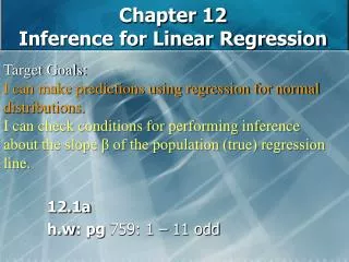
The Regression Model • We have learned that when a scatterplot shows a linear relationship between a quantitative explanatory variable x and a quantitative response variable y, we can use the least-squares regression line fitted to the data to predict y for a given value of x. • Now, we want to do tests and confidence intervals in this setting.
Crying and IQ • Infants who cry easily may be more easily stimulated than others. This may be a sign of higher IQ. Child development researchers explored the relationship between the crying of infants four to ten days old and their later IQ test scores. A snap of a rubber band on the sole of the foot caused the infants to cry. The researchers recorded the crying and measured its intensity by the number of peaks in the most active 20 seconds. They later measured the children’s IQ at age three years using the Stanford-Binet IQ test. The data for 38 infants are given on the next slide.
Crying and IQ • Who? – All we know is that the individuals are 38 infants who were studied when they were 4 to 10 days old and then again when they were 3 years old. • What? – The explanatory variable is crying intensity and the response variable is children’s IQ. • Why? – Researchers wanted to see if there is an association between crying activity in early infancy and IQ at age 3 years. • When, where, how, and by whom? – The data come from an experiment described in 1964 in the journal Child Development.
Crying and IQ • As always, we start with a graphical display of the data, in this case a scatterplot. • What are the form, direction and strength of the relationship as well as any deviations from the pattern (outliers, influential observations) in the scatterplot? • From the scatterplot, there appears to be a moderate positive linear relationship with no extreme values or influential observations. • To get a better idea of the strength, we find that r is 0.455 for our data. This confirms a moderate positive association. What is r2 and what does it tell us?
Crying and IQ • The least-squares regression line of IQ scores (y) on crying intensity (x) is given by the equation • Since r2 is 0.207, only about 21% of the variation of IQ scores is explained by crying intensity. • Therefore, prediction of IQ scores from crying intensity will not be very accurate.
Conditions for the Regression Model • The slope b and y-intercept a of the least-squares line are statistics. That is, we calculate them from sample data. • To do formal inference, we think of a and b as estimates of unknown parameters. • The conditions for performing inference are on the next slide.
The idea is shown in the graph on the next page. The basic idea is that we expect y values to vary according to a normal distribution.
As you can see, the y values are centered on the true regression line for the population and vary according to a Normal distribution.
Checking Conditions • The observations must be independent. In particular, we cannot use repeated observations on the same individual. • The true relationship is linear. We can’t observe the true regression line, so we will almost never see a perfectly straight line. So we look at the scatterplot and a residual plot to make sure that a line appears to be a good fit. • The standard deviation of the response variable about the true line is the same everywhere. Looking at the scatterplot again, the scatter of the data points about the line should be roughly the same over the range of all the data. Looking at a residual plot is another way to do this.
Checking Conditions • The response varies Normally about the true regression line. We can’t observe the true regression line. What we can observe is the least-squares regression line and the residuals. The residuals estimate the deviations of the response from the true regression line, so they should follow a Normal distribution. Make a histogram or stemplot of the residuals and check for clear skewness or other major departures from Normality. It turns out that inference for regression is not very sensitive to a minor lack of Normality, especially when we have many observations. Do beware of influential points which move the regression line and can greatly affect the results of inference.
Checking Conditions • Fortunately, it is not hard to check for gross violations of these conditions for regression inference. • Since checking conditions uses residuals, most regression software will calculate and save the residuals for you. • We will talk about how to have the calculator find the residuals for you on the next slide.
Calculating Residuals • Go to your lists. • Go up to where the listname is (L1, L2, etc.). • Now, scroll to your right until you get a list with no name, just dashes. • Now, hit 2nd and then Stat to go to all lists. • Scroll down and highlight beside RESID and hit enter. • Hit enter one more time and it is now there. • Now, every time you do a regression, the residuals will automatically be listed here for you.
Crying and IQ • Let’s find the residuals for our data. • To do this, we just need to run a linear regression on our data and the residuals will automatically be stored in RESID for us. • The 38 residuals are listed below. • Now, let’s create a residual plot. So plot L1 against RESID. • Now, let’s see if the residuals appear Normally distributed. To do this, look at a boxplot and a histogram. The book used a stemplot.
Crying and IQ • Based on what we looked at, the pattern appears to fairly linear since there is no pattern to the residual plot. • The residuals also appear to be approximately Normally distributed. There is some slight right-skewness, but we see no serious violations of our conditions.
Estimating the Parameters • The first step in inference is to estimate the unknown parameters α, β, and σ. • When the regression model describes our data and we calculate the least-squares regression line, the slope of the regression line, b, is an unbiased estimator of the true slope β and the intercept a is an unbiased estimator of the true intercept α.
Estimating the Parameters • The remaining parameter of the model is the standard deviation σ, which describes the variability of the response y about the true regression line. • The least-squares regression line estimates the true regression line. So the residuals estimate how much y varies about the true line. • There are n residuals, one for each data point. Because σ is the standard deviation of responses about the true regression line, we estimate it by a sample standard deviation of the residuals.
Estimating the Parameters • We call this sample standard deviation a standard error to emphasize that it is estimated from data. • Notice that we divide by n – 2 rather than n – 1. This is because we have n – 2 degrees of freedom.
Crying and IQ • For our data, we get an LSRL of • The true slope would tell us how much higher IQ would get when the number of peaks in their crying measurements increased by 1. • For our example, we are estimating the slope β to be 1.493. In other words, IQ is about 1.5 points higher for each additional crying peak. • We also estimate the y-intercept α to be 91.27. This has no statistical meaning though because the value is outside of our x values in the problem. Our smallest x value is 9. Also, it is reasonable to believe that all babies would cry if hit with a rubber band.
Crying and IQ • Now we want to find s. • To do this, we need to know the residuals. They should be in the list RESID. • Since we need to find the sum of the squares of the residuals • We can do this by typing the following in our calculator We get 17.499 for s. • We can also find s by going to TESTS and selecting F: LinRegTTest. Scroll down and find s. Notice we also get 17.499 for s.
Confidence Intervals for the Regression Slope • The slope β of the true regression line is usually the most important parameter in a regression problem. • The slope is the rate of change of the mean response as the explanatory variable increases. • We often want to estimate β. The slope b of the LSRL is an unbiased estimator of β. • A confidence interval for β is useful because it shows how accurate the estimate b is likely to be. • This confidence interval will have the familiar form:
Confidence Intervals for the Regression Slope • Because our estimate is b, the confidence interval becomes • Here are the details.
Crying and IQ • We can create a 95% confidence interval using the printout above. • We can find t* from the table or on the calculator. I used the calculator. Go back!
Crying and IQ • We are going to learn in a little while that • We need to know this to calculate the interval by hand. • Going to LinRegTTest, we can find t and b. This allows us to find SEb. • From the calculator, t = 3.0655 and b = 1.4929. • So • Therefore, the 95% C.I. is
Testing the Hypothesis of No Linear Relationship • The most common hypothesis about the slope is • A regression line with slope 0 is horizontal. That is, the mean of y does not change at all when x changes. So this H0 says that there is no true linear relationship between x and y. • Put another way, H0 says that there is no correlation between x and y in the population from which we drew our data. • You can use the test for zero slope to test the hypothesis of zero correlation between any two quantitative variables.
Testing the Hypothesis of No Linear Relationship • Notice that testing correlation makes sense only if the observations are a random sample. This is often not the case in regression settings, where researchers may fix in advance the values of x they want to study. • The statistic again takes the form • The test statistic is just the standardized version of the least-squares regression slope b. • The details are on the next slide.
Notice that the numerator is just b because we usually test that the parameter is equal to 0.
Crying and IQ • Let’s revisit our example. • What are our t value and p-value? • How could we find these on the calculator? • What would we have to show on the AP Exam? • Where did these numbers come from? • The calculator gives us b and t, so we use that to find SEb.
Beer and Blood Alcohol Content • We are going to revisit our beer and blood alcohol content example from Chapter 3. • The number of beers a volunteer drank and their recorded BAC are given in the table below. • We want to conduct a significance test. We believe that drinking more beer will increase the BAC.
Beer and Blood Alcohol Content • Step 1: Hypotheses • Step 2: Conditions for a Linear Regression t Test • Each observation is independent of the others. • The scatterplot is reasonably linear and the residual plot does not indicate that the data is not linear. This indicates that the true relationship is linear. • The residual plot does not provide any reason to believe that the standard deviation of the responses about the true line are not the same everywhere. • Looking at a histogram or boxplot of the residuals, we can see that the residuals are skewed right, but there are no major departures from Normality for a sample this small.
Beer and Blood Alcohol Content • Step 3: Calculations • Step 4: Interpretation • Since our p-value of 0.000001 is smaller than any standard significance level, we reject H0. We therefore conclude that there is very strong evidence that increasing the number of beers does increase BAC.
Beer and Blood Alcohol Content • Let’s create a 99% C.I. just to review. We have already done Steps 1 and 2. • t* with df = 14 would be 2.977. • Since the calculator gives us t and b, we can find SEb. • So • Hence, the 99% C.I. would be
Testing other than Slope of 0 • Suppose we want to test the following for the data below. • The calculations are the only part that is different. They appear on the next slide.
Testing other than Slope of 0 • Calculations • Now • Where did SEb come from? • Since the calculator gives us t and b when we do a LinRegTTest, we still use this to find SEb. Then we just plug into the formula and find our own t value for the slope other than 0. • P-value = 0.8577. How did we find it? • 2 tcdf (0.1819, 10000000000, 18) • Why did we multiply by 2? • So we fail to reject. There is not enough evidence to believe that the slope is not equal to 1.
Crying and IQ Go back!
Crying and IQ Go back!
Crying and IQ Go back!
Minitab Output of Beers vs. BAC • A word of warning. Computer output always gives a two-sided p-value. So if you are finding the p-value for a one-sided test, you need to divide the p-value by 2. Go back!
Scatterplot of Beers vs. BAC Go back!
Residual Plot of Beers vs. BAC Go back!