Download
1 / 32
320 likes | 332 Views
This algorithm iteratively estimates the structure of populations by counting recombination events and allows for admixture mapping. It uses a sampling approach to estimate the admixture probability and assigns individuals to sub-populations based on linkage equilibrium and Hardy Weinberg equilibrium. The algorithm also provides estimates of recombination rates and uses lower bounds to compute the minimum number of recombination events in a population. The results on simulated and real data show the effectiveness of the algorithm in predicting population structure and admixture.

E N D
Algorithm:Structure • Iteratively estimate • (Z(0),P(0)), (Z(1),P(1)),.., (Z(m),P(m)) • After ‘convergence’, Z(m) is the answer. • Iteration • Guess Z(0) • For m = 1,2,.. • Sample P(m) from Pr(P | X, Z(m-1)) • Sample Z(m) from Pr(Z | X, P(m)) • How is this sampling done?
Allowing for admixture • Define qi,k as the fraction of individual i that originated from population k. • Iteration • Guess Z(0) • For m = 1,2,.. • Sample P(m),Q(m) from Pr(P,Q | X, Z(m-1)) • Sample Z(m) from Pr(Z | X, P(m),Q(m))
Estimating Z (admixture case) • Instead of estimating Pr(Z(i)=k|X,P,Q), (origin of individual i is k), we estimate Pr(Z(i,j,l)=k|X,P,Q) i,1 i,2 j
Results: Thrush data • For each individual, q(i) is plotted as the distance to the opposite side of the triangle. • The assignment is reliable, and there is evidence of admixture.
Population Structure • 377 locations (loci) were sampled in 1000 people from 52 populations. • 6 genetic clusters were obtained, which corresponded to 5 geographic regions (Rosenberg et al. Science 2003) Oceania Eurasia East Asia America Africa
NJ versus Structure:thrush data • Objective function is different in standard clustering algorithms!
Population sub-structure:research problem • Systematically explore the effect of admixture. Can admixture be predicted for a locus, or for an individual • The sampling approach may or may not be appropriate. Formulate as an optimization/learning problem: • (w/out admixture). Assign individuals to sub-populations so as to maximize linkage equilibrium, and hardy weinberg equilibrium in each of the sub-populations • (w/ admixture) Assign (individuals, loci) to sub-populations
Recombination in human chromosome 22 (Mb scale) Dawson et al. Nature 2002 Q: Can we give a direct count of the number of the recombination events?
Recombination rates (chimp/human) • Fine scale recombination rates differ between chimp and human • The six hot-spots seen in human are not seen in chimp
Combinatorial Bounds for estimating recombination rate • Recall that expected #recombinations = log n • Procedure • Generate N random ARGs that results in the given sample • Compute mean of the number of recombinations • Alternatively, generate a summary statistic s from the population. • For each , generate many populations, and compute the mean and variance of s (This only needs to be done once). • Use this to select the most likely • What is the correct summary statistic? • Today, we talk about the min. number of recombination events as a possible summary statistic. It is not the most natural, but it is the most interesting computationally.
The Infinite Sites Assumption & the 4 gamete condition 0 0 0 0 0 0 0 0 3 0 0 1 0 0 0 0 0 5 8 0 0 1 0 1 0 0 0 0 0 1 0 0 0 0 1 • Consider a history without recombination. No pair of sites shows all four gametes 00,01,10,11. • A pair of sites with all 4 gametes implies a recombination event
Hudson & Kaplan • Any pair of sites (i,j) containing 4 gametes must admit a recombination event. • Disjoint (non-overlapping) sites must contain distinct recombination events, which can be summed! This gives a lower bound on the number of recombination events. • Based on simulations, this bound is not tight.
Myers and Griffiths’03: Idea 1 • Let B(i,j) be a lower bound on the number of recombinations between sites i and j. 1=i1 i2 i3 i4 i5 i6 ik=n • Can we compute maxP R(P) efficiently?
Improved lower bounds • The Rm bound also gives a general technique for combining local lower bounds into an overall lower bound. • In the example, Rm=2, but we cannot give any ARG with 2 recombination events. • Can we improve upon Hudson and Kaplan to get better local lower bounds? 0 0 0 0 0 1 0 1 0 0 1 1 1 0 0 1 0 1 1 1 0 1 1 1
Hudson and Kaplan: Idea 2 • Consider the history of individuals. Let Ht denote the number of distinct halotypes at time t • One of three things might happen at time t: • Mutation: Ht increase by at most 1 • Recombination: Ht increase by at most 1 • Coalescence: Ht does not increase
The RH bound 0 0 0 0 0 1 0 1 0 0 1 1 1 0 0 1 0 1 1 1 0 1 1 1 Ex: R>= 8-3-1=4
RH bound • In general, RH can be quite weak: • consider the case when S>H • However, it can be improved • Partitioning idea: sum RH over disjoint intervals • Apply to any subset of columns. Ex: Apply RH to the yellow columns 000000000000000 000000000000001 000000010000000 000000010000001 100000000000000 100000000000001 100000010000000 111111111111111 (BB’05)
The Rs bound • Compute the minimum number of recombination events R in any ARG. Note that, we do not explicitly construct the ARG. • Consider a matrix with M with H rows and S columns. • The rows correspond to haplotypes. • Columns correspond to sites.
a b c Rs bound: Observation I s • Non-informative column: If a site contains at most one 1, or one 0, then in any history, it can be obtained by adding a mutation to a branch. • EX: if a is the haplotype containing a 1, It can simply be added to the branch without increasing number of recombination events • R(M) = R(M-{s}) 0 0 0 : : 1 a
Rs bound: Observation 2 • Redundant rows: If two rows h1 and h2 are identical, then • R(M) = R(M-{h1}) c r1 r2
Rs bound: Observation 3 • Suppose M has no non-informative columns, or redundant rows. • Then, at least one of the haplotypes is a recombinant. • There exists h s.t. R(M) = R(M-{h})+1 • Which h should you choose?
Rs bound (Procedural) Procedure Compute_Rs(M) If non-informative column s return (Compute_Rs(M-{s})) Else if redundant row h return (Compute_Rs(M-{h})) Else return (1 + minh(Compute_Rs(M-{h}))
Additional results/problems • Using dynamic programming, Rs can be computed in 2^n poly(mn) time. • Also, Rs can be augmented to handle intermediates. • Are there poly. time lower bounds? • The number of connected components in the conflict graph is a lower bound (BB’04). • Fast algorithms for computing ARGs with minimum recombination. • Poly. Time to get ARG with 0 recombination • Poly. Time to get ARGs that are galled trees (Gusfield’03)
Underperforming lower bounds • Sometimes, Rs can be quite weak • An RI lower bound that uses intermediates can help (BB’05)
LPL data set • 71 individuals, 9.7Kbp genomic sequence • Rm=22, Rh=70