Download

1 / 24
240 likes | 260 Views
This study focuses on the diurnal variation of the geomagnetic field and how it can be used to reconstruct the solar extreme ultraviolet (EUV) flux from 1740 to 2015. By analyzing reliable magnetic data, the conductivity and EUV flux can be deduced, providing insights into solar activity over centuries.

E N D
Reconstruction of Solar EUV Flux 1740-2015 Leif Svalgaard Stanford University AGU, Fall SA51B-2398, 2015
The Diurnal Variation of the Direction of the Magnetic Needle 10 Days of Variation George Graham [London] discovered [1722] that the geomagnetic field varied during the day in a regular manner.
Balfour Stewart, 1882, Encyclopedia Britannica, 9th Ed. “The various speculations on the cause of these phenomena [daily variation of the geomagnetic field] have ranged over the whole field of likely explanations. (1) […], (2) It has been imagined that convection currents established by the sun’s heating influence in the upper regions of the atmosphere are to be regarded as conductors moving across lines of magnetic force, and are thus the vehicle of electric currents which act upon the magnet, (3) […], (4) […]. Balfour Stewart 1828-1887 “there seems to be grounds for imagining that their conductivity may be much greater than has hitherto been supposed.”
Dynamo Ionospheric Layers An effective dynamo process takes place in the dayside E-layer where the density, both of the neutral atmosphere and of the electrons are high enough. We thus expect the geomagnetic response due to electric currents induced in the E-layer.
The E-layer Current System North X . rY Morning H rD Evening D East Y Y = H sin(D) dY = H cos(D) dD For small dD A current system in the ionosphere is created and maintained by solar EUV radiation The magnetic effect of this system was what George Graham discovered
The Physics With the possible exception of the ‘solar boxes’ the physics of the rest of the boxes is well-understood We’ll be concerned with deriving the EUV flux from the observed diurnal variation of the geomagnetic field
Electron Density due to EUV The conductivity at a given height is proportional to the electron number density Ne. In the dynamo region the ionospheric plasma is largely in photochemical equilibrium. The dominant plasma species is O+2, which is produced by photo ionization at a rate J (s−1) and lost through recombination with electrons at a rate α (s−1), producing the Airglow. < 102.7 nm The rate of change of the number of ions Ni, dNi/dt and in the number of electrons Ne, dNe/dt are given by dNi/dt = J cos(χ) - αNiNe and dNe/dt = J cos(χ) - αNeNi. Because the Zenith angle χchanges slowly we have a quasi steady-state, in which there is no net electric charge, so Ni = Ne = N. In a steady-state dN/dt = 0, so the equations can be written 0 = J cos(χ) - αN2, and so finally N =√(Jα-1cos(χ)) Since the conductivity, Σ, depends on the number of electrons N, we expect that Σ scales with the square root √(J) of the overhead EUV flux with λ < 102.7 nm.
Solar Cycle and Zenith Angle Control Johann Rudolf Wolf, 1852 + J-A. Gautier EUV
The Diurnal Variation of the Declination for Low, Medium, and High Solar Activity
PSM-POT-VLJ-SED-CLF-NGK A ‘Master’ record can now be build by averaging the German and French chains. We shall normalize all other stations to this Master record.
Adding Prague back to 1840 If the regression against the Master record is not quite linear, a power law is used.
N Std Dev.
Composite rY Series 1840-2014 From the Standard Deviation and the Number of Station in each Year we can compute the Standard Error of the Mean and plot the ±1-sigma envelope. Of note is the constancy of the range at every sunspot minimum
EUV and its proxy: F10.7 Microwave Flux F10.7 Space is a harsh environment: Sensor Degradation
rY and F10.71/2 and EUV1/2 √(J) Since 1996 Since 1996 Since 1947
Agreement across UV spectrum The Bremen Mg II (λ = 280 nm) Index composite (courtesy Mark Weber) has very high correlation (R2 = 0.98, yearly) with our rY composite. Scaling the Mg II index and the (bit more noisy) NSO Ca II K-line index (λ = 393 nm) to the Diurnal Range, rY, shows that all three indices agree well over the range from EUV to low-λ visible.
Reconstructed EUV Flux 1840-2014 This is, I believe, an accurate depiction of ‘true’ solar activity since 1840
We Can Go Further Back Lovö magnetic obs. April 1997 Olof Peter Hjorter
Abstract Solar Extreme Ultraviolet (EUV) radiation creates the conducting E–layer of the ionosphere, mainly by photo ionization of molecular Oxygen. Solar heating of the ionosphere creates thermal winds which by dynamo action induce an electric field driving an electric current having a magnetic effect observable on the ground, as was discovered by G. Graham in 1722. The current rises and sets with the Sun and thus causes a readily observable diurnal variation of the geomagnetic field, allowing us the deduce the conductivity and thus the EUV flux as far back as reliable magnetic data reach. High–quality data go back to the ‘Magnetic Crusade’ of the 1830s and less reliable, but still usable, data are available for portions of the hundred years before that. J.R. Wolf and, independently, J.–A. Gautier discovered the dependence of the diurnal variation on solar activity, and today we understand and can invert that relationship to construct a reliable record of the EUV flux from the geomagnetic record. We compare that to the F10.7 flux and other solar indices, and find that the reconstructed EUV flux reproduces the F10.7 flux with great accuracy. The reconstruction suggests that the EUV flux reaches the same non–zero value at every sunspot minimum (possibly including Grand Minima), representing an invariant ‘solar magnetic ground state’.