Download
1 / 34
340 likes | 443 Views
Learn basic terminology and methods for fitting a line to bivariate data. Explore how to determine the "best" line using least squares and evaluating the usefulness of the least squares line. Discover the concept of residuals and their importance in linear regression analysis. Practice through examples like Fuel Consumption vs Car Weight.

E N D
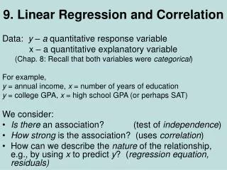
Chapters 8, 9, 10Linear Regression Fitting a Line to Bivariate Data
Basic Terminology • Explanatory variable: explains or causes changes in the other variable; the x variable. (independent variable) • Response variable: the y -variable; it responds to changes in the x - variable. (dependent variable)
Simplest Relationship • Simplest equation that describes the dependence of variable y on variable x y = b0 + b1x • linear equation • graph is line with slope b1 and y-intercept b0
Graph y=b0 +b1x y rise Slope b=rise/run b0 run 0 x
Notation • (x1, y1), (x2, y2), . . . , (xn, yn) • draw the line y= b0 + b1x through the scatterplot , the point on the line corresponding to xi is
Observed y, Predicted y predicted y when x=2.7 = b0 + b1x = b0 + b1*2.7 2.7
Scatterplot: Fuel Consumption vs Car Weight “Best” line?
Criterion for choosing what line to draw: method of least squares • The method of least squares chooses the line that makes the sum of squares of the residuals as small as possible • This line has slope b1 and intercept b0 that minimizes
Car Weight, Fuel Consumption Example, cont. (xi, yi): (3.4, 5.5) (3.8, 5.9) (4.1, 6.5) (2.2, 3.3) (2.6, 3.6) (2.9, 4.6) (2, 2.9) (2.7, 3.6) (1.9, 3.1) (3.4, 4.9)
The Least Squares Line Always goes Through ( x, y ) (x, y ) = (2.9, 4.39)
Using the least squares line for prediction. Fuel consumption of 3,000 lb car? (x=3)
Be Careful! Fuel consumption of 500 lb car? (x = .5) x = .5 is outside the range of the x-data that we used to determine the least squares line
Avoid GIGO! Evaluating the least squares line • Create scatterplot. Approximately linear? • Calculate r2, the square of the correlation coefficient • Examine residual plot
r2 : The Variation Accounted For • The square of the correlation coefficient r gives important information about the usefulness of the least squares line
r2: important information for evaluating the usefulness of the least squares line -1 ≤ r ≤ 1 implies 0 ≤ r2 ≤ 1 The square of the correlation coefficient, r2, is the fraction of the variation in y that is explained by the least squares regression of y on x. The square of the correlation coefficient, r2, is the fraction of the variation in y that is explained by differences in x.
March Madness: S(k) Sagarin rating of kth seeded team; Yij =Vegas point spread between seed i and seed j, i<j 94.8% of the variation in point spreads is explained by the variation in Sagarin rating differences
SAT scores: result r2 = (-.86845)2= .7542 Approx. 75.4% of the variation in mean SAT math scores is explained by differences in the percent of seniors taking the SAT.
Avoid GIGO! Evaluating the least squares line • Create scatterplot. Approximately linear? • Calculate r2, the square of the correlation coefficient • Examine residual plot
Residuals • residual =observed y - predicted y = y - y • Properties of residuals • The residuals always sum to 0 (therefore the mean of the residuals is 0) • The least squares line always goes through the point (x, y)
Graphicallyresidual = y - y y yi yi ei=yi - yi X xi
Residual Plot • Residuals help us determine if fitting a least squares line to the data makes sense • When a least squares line is appropriate, it should model the underlying relationship; nothing interesting should be left behind • We make a scatterplot of the residuals in the hope of finding… NOTHING!
Residuals: Sagarin Ratings and Point Spreads Yij Predicted Yij Residuals 20 23.48573586 -3.485735859 24 21.3717734 2.628226598 18 13.96719139 4.032808608 11 11.52185104 -0.521851036 6 5.774158519 0.225841481 8.5 7.613877198 0.886122802 4 1.683355495 2.316644505 4 2.186135755 1.813864245 28 27.26801463 0.731985367 16 15.53266629 0.467333708 11.5 10.56199781 0.938002187 12 10.11635167 1.883648327 4 5.397073324 -1.397073324 7 6.836853159 0.163146841 -1.5 1.500526309 -3.000526309 2 1.946172449 0.053827551 Yij Predicted Yij Residuals 25 23.58857728 1.411422725 18.5 18.34366502 0.156334982 10.5 12.85878945 -2.358789455 11.5 10.95050983 0.549490168 4.5 2.597501422 1.902498578 5 6.631170326 -1.631170326 4 3.203123099 0.796876901 -3.5 0.095026946 -3.595026946 23 24.15991848 -1.15991848 20.5 21.24607834 -0.746078337 18 20.0919691 -2.091969104 10.5 11.62469245 -1.124692453 9 6.836853159 2.163146841 7 5.979841353 1.020158647 2 3.283110867 -1.283110867 5 6.745438567 -1.745438567